Lab 03: A time constant in silicon
You designed a resistor in Lab 01 and a capacitor in Lab 02. In this lab you’ll put them in one circuit and measure its time constant, learn to tell a measurement artefact from a real device effect, and find the split between \(R\) and \(C\) that gives a target \(\tau\) in the least area. Then you’ll measure the same RC in the frequency domain, and see why chips time long intervals by counting clock ticks rather than by charging a capacitor.
Package: labs/lab-03-a-time-constant-in-silicon/
Before you start
Finish Lab 01 and Lab 02. This lab uses the resistor (\(L = 30.3315\) µm) and capacitor (\(s = 22.1965\) µm) you sized there, and Lab 01’s
solutions/README.md.Open a terminal in the workbench and go to the lab folder:
cd /foss/designs/modules/ad102/labs/lab-03-a-time-constant-in-siliconThe decks don’t need any environment setup. Only the XSchem window in the optional Part 8 needs the noVNC desktop and
$PDKset tosky130A(Lab 01, Part 1).
Parts 1 to 7 are required. Part 8, under Going further at the end, is optional.
Time: about 2 hours, not counting the optional part. make runs two ngspice decks, and each one prints nothing while the SKY130 model cards load, which takes about a minute per deck on the pinned image (see Warnings and delays).
A resistor charging a capacitor from a step follows
\[v(t) = V_f\left(1 - e^{-t/RC}\right) \qquad \tau = RC\]
At \(t = \tau\) the output has covered \(1 - e^{-1} = 0.632120\) of the way to its final value. So to measure \(\tau\) you step the input and find the moment the output crosses 63.2 % of its final value; that time is \(\tau\) by definition. Every meas in this lab is a single line that does exactly this.
Part 1: Measure two time constants you can predict
Does a meas on a simple RC return the \(\tau\) you predict?
Section A of spice/rc.spice is ECE334’s lab-1 RC deck, unchanged: a 1 kΩ/2 kΩ divider with 0.7 pF on the tap, driven by a 1.8 V pulse. If you’re a UofT student, it’s probably a version of this circuit you have already run. Section B is an ideal 10 kΩ and an ideal 1 pF, so its \(\tau\) is 10 ns by construction.
Predict both time constants. In section A the capacitor charges through the Thévenin resistance of the divider rather than through the 1 kΩ alone:
\[R_{\text{th}} = 1\text{k} \parallel 2\text{k} = 666.67\ \Omega \qquad \tau = 666.67 \times 0.7\,\text{pF} = 466.67\ \text{ps}\]
and it charges toward \(1.8 \times \tfrac{2}{3} = 1.2\) V.
Run the lab:
makeIt ends in
FAILbecause of area, which you’ll fix in Part 6. Leave the output in your terminal.Read the raw
measlines near the top of the output, rather than the checker’s table:t_ece334 = 1.47167e-09 t_ideal = 1.10050e-08 v_ece334 = 1.20000e+00The step happens at \(t = 1\) ns, so subtract 1 ns from each time and compare with your predictions.
You should see: a final value of 1.2000 V, as Thévenin predicts. The times are slightly off, though: the ECE334 circuit took 471.67 ps against a predicted 466.67, and the ideal RC took 10.0050 ns against a predicted 10.0000. Both are 5 ps late, even though their time constants differ by a factor of twenty-one.
An error that stays the same size whatever you measure can’t be coming from the thing you’re measuring, so look at what the two circuits have in common. The pulse source in the deck is
Va ai 0 PULSE(0 1.8 1n 10p 10p 200n 400n)Where do the 5 ps come from?
The rise time is 10 ps, so the step is really a ramp, and a first-order system responds as though the step arrived at the ramp’s midpoint, which is 5 ps after the ramp starts. check_rc.py subtracts 1.005 ns instead of 1 ns, and then both circuits read exactly right:
  A  ECE334 deck: 1k/2k divider + 0.7 pF, ideal         466.6700 ps    466.6700 ps
  B  ideal 10 kohm + ideal 1 pF                          10.0000 ns     10.0000 ns
Telling a measurement artefact from a device effect is most of what analog verification is, and the clue here was that the error didn’t scale with \(\tau\).
Part 2: Swap in your own resistor and capacitor
Does the RC still give 10 ns when the parts are the ones you designed?
Sections C, D and E of the deck replace the ideal 10 kΩ with your Lab 01 resistor (\(L = 30.3315\) µm), then the ideal 1 pF with your Lab 02 capacitor (\(s = 22.1965\) µm), then both.
Predict all three. You designed both devices to hit their targets to better than one part in ten thousand, so your prediction should be 10.0000 ns each time.
Find lines C, D and E in the checker’s table.
Find section H in the raw output, the block headed
--- H. the resistor's own capacitance to substrate. It leaves the far end of each resistor unconnected and measures the current the source still has to supply, and from that current it works out the resistor’s own capacitance to the substrate.
You should see:
  C  YOUR Lab 01 resistor + ideal 1 pF                   10.0361 ns
  D  ideal 10 kohm + YOUR Lab 02 capacitor               10.0000 ns
  E  both of yours, no ideal parts anywhere              10.0362 ns
--- H. the resistor's own capacitance to substrate (farads) ---
cpar_10k = 7.233642e-15
cpar_1m = 9.527372e-14Your capacitor makes no difference: replacing the ideal 1 pF with a real MIM plate changes nothing to five figures. Your resistor adds 36.1 ps, and it adds the same 36.1 ps whether the capacitor next to it is real or ideal. The checker fits a line through the two strips from section H and prints the result below its table:
fitting both strips: 0.1994 fF per um of 1 um-wide poly, plus 1.1869 fF of ends.You’ll use that 0.1994 fF per µm in Parts 5 and 6.
How does section H account for the 36 ps?
A 30 µm strip of poly is also a 7.2 fF capacitor, whether you wanted one or not. For a distributed RC line, half of that capacitance adds to the time constant: \(10\,\text{k}\Omega \times 7.234\,\text{fF}/2 = 36.2\) ps, against the 36.1 ps you measured. At 10 kΩ this costs you 0.36 %, and Part 5 finds the size of resistor where you can no longer ignore it.
Part 3: Sizing without Labs 01 and 02
What would this circuit have done if you had sized it from the model cards alone?
Section F sizes the same circuit with the two naive rules: the resistor’s length comes straight from the sheet resistance, and the capacitor’s area straight from the capacitance density.
In Lab 01 the end resistance was worth 3.7 % on a 10 kΩ resistor, and in Lab 02 the fringe was worth 1.5 % on a picofarad. Predict the timing error of the naively sized circuit.
Find line F and the two summary lines below the table.
You should see:
  F  the same circuit sized without Labs 01 and 02       10.5647 ns

  designing with Labs 01 and 02 : +0.36 % from the 10.0000 ns you asked for
  designing without them        : +5.65 %
Together with the resistor’s own 0.36 % from Part 2, the two sizing errors add up to 5.65 % of timing error in one circuit. Neither of them shows up as a warning or in DRC, and neither averages out across a wafer, because every chip gets the same 5.65 %. That’s the difference Lab 01, Part 3 drew between a tolerance, which you budget for, and a mistake, which you don’t know is there.
Part 4: Temperature
How much does the same silicon drift between −40 °C and +125 °C?
The deck runs section E again at −40 °C and at +125 °C, with no change to the layout.
Predict the direction before you look. Lab 01’s
solutions/README.mdgaveres_high_po’s temperature coefficient astc1 = 0.514e-3.Find the two “E again” lines and the span line.
You should see:
     E again at -40 C                                     9.7849 ns
     E again at +125 C                                   10.6544 ns

  and the SAME silicon over -40 C to +125 C spans 8.66 %
You’ve spent this lab chasing a 5.65 % sizing error, and temperature on its own is worth 8.66 % over an industrial range. The MIM capacitor’s model card has tc1 = 0. What does that tell you about where the drift comes from, and about using an on-chip RC as a clock?
The MIM capacitor contributes almost none of the drift, so nearly all of it comes from the resistor. An on-chip RC is a fine way to set a filter corner that is allowed to wander, and a bad way to make a clock.
Part 5: A one-microsecond RC
What happens to a real RC when the resistor gets big?
Section G of the deck builds a 1 µs RC twice: once with an ideal 1 MΩ, and once with a real one made of 471.96 µm of res_xhigh_po, sized with your Lab 01 numbers. The checker’s table calls these two G and H.
Using the 0.1994 fF per µm from Part 2, predict the error before you look.
Find lines G and H in the checker’s table, and the lines about the microsecond below it. (This H is the checker’s line, not section H of the raw output, which you read in Part 2.)
You should see:
  G  ideal 1 Mohm + ideal 1 pF                          999.9950 ns
  H  real 1 Mohm of xhigh poly + your 1 pF             1049.8950 ns

  the microsecond ran 49.90 ns long.
    a 471.96 um strip of poly carries 95.274 fF to the substrate, and half of it
    adds to the time constant: R*Cpar/2 = 47.64 ns, which is 95 % of what you measured.
The microsecond runs 5 % long without any capacitor being mis-sized, because the strip that makes the megohm carries 95 fF of its own, about a tenth of the capacitor it is charging.
A millisecond needs a thousand times this \(RC\), say 100 MΩ and 10 pF. Could you build it?
No. At 1 µm wide, 100 MΩ of res_xhigh_po is 47,197 µm of poly, which is 4.7 centimetres folded into a serpentine, and it carries about 9.4 pF to the substrate by itself. The resistor’s parasitic is then about the same size as the capacitor it was supposed to charge, and no choice of either value fixes that.
So you can’t build a millisecond from an RC on a chip. What chips do instead is count: an oscillator makes a short, repeatable interval, and a digital counter multiplies it. That’s why DD103’s elevator controller measures its door dwell in clock ticks. It’s one of the cleanest examples anywhere of a digital answer to an analog question, and this measurement shows you why the question comes up.
Part 6: Your own 20 ns time constant
How small can you make a 20 ns RC?
spice/my_rc.spice has one resistor length and one capacitor side for you to choose. Your job is to build a 20.0 ns time constant, within 1 %, in under 400 µm² of drawn area.
The file ships with 2 kΩ and 10 pF. That gives a perfectly good 20 ns, but it costs 4981.84 µm², twelve times the budget, which is why the check in Part 1 failed on area rather than on timing:
  resistor  L =   5.1124 um at W = 1 um   ->       5.11 um^2
  capacitor s =  70.5459 um square       ->    4976.72 um^2
  total drawn area                         ->    4981.84 um^2   (budget 400)   FAIL
  tau = 20.0020 ns   target 20.0000 ns   (+0.01 %)   PASS
Write down the two sizing formulas you already have, and the area:
\[R = 378.2448 + 317.2198\,L \qquad C[\text{fF}] = 2.000000\,s^2 + 0.659991\,s - 0.017742\]
Area is \(L + s^2\).
Work out which way to move \(R\) and \(C\) to reduce the area while keeping \(RC = 20\) ns, and find the optimum.
Account for the resistor’s own parasitic, which from Part 2 is 0.1994 fF per micrometre of length plus 1.187 fF for the ends. As the capacitor gets smaller, the parasitic becomes a visible fraction of it and \(\tau\) runs long, because half of the parasitic adds to the capacitor: \(\tau \approx R\,(C + C_{\text{par}}/2)\). Make the capacitor you draw smaller by enough to make up for it.
In
spice/my_rc.spice, change the resistor’sL=and the capacitor’sW=andL=(keeping the plate square). Write them as plain microns with nousuffix, then re-run:make mine check
You should see: both the area line and the tau line marked PASS, then
PASS -- every number matches the reference run.Part 7: The same RC in the frequency domain
Does the corner frequency from an .ac analysis agree with the \(\tau\) you measured?
So far you have measured the RC the way you would with a stopwatch, by stepping the input and timing the output. AD101 taught the other way, which is to drive the input at every frequency and find where the output stops keeping up. The two answers are tied together by
\[f_{-3\text{dB}} = \frac{1}{2\pi\tau}\]
spice/bode.spice uses the same two devices as section E, and also simulates an ideal 10 kΩ and an ideal 1 pF, the same pair as section B of rc.spice, for comparison.
Take your \(\tau\) from Part 2, 10.0362 ns, and predict the corner frequency.
Run the frequency-domain deck and draw its plot:
make bodeIt loads the same model library as the other decks, so expect the same wait.
You should see:
f3db_real           =  1.58580e+07
f3db_ideal          =  1.59155e+07
ph_real             =  -7.85359e-01
--- decade of roll-off: the real filter, dB at 10x the corner ---
g_10x               =  -2.00426e+01
  wrote results/ad102-rc-bode.png
That PNG is your own copy of the figure below, drawn from your own results/bode.txt.
Your prediction was
\[\frac{1}{2\pi \times 10.0362\ \text{ns}} = 15.858088\ \text{MHz}\]
and .ac measured 15.8580 MHz. They agree to five significant figures, about six parts per million apart, from two analyses that share nothing but the two device lines. Agreement between two independent measurements is the only evidence you get that a deck is right, and checking one against the other costs nothing, so make a habit of it. With any RC you have three numbers, \(R\), \(C\) and \(\tau\), and any two of them give you the third. If they disagree, one of your decks is wrong, and you’ve found out cheaply.
The other two lines confirm the shape of a first-order filter:
ph_real = -7.85359e-01is in radians. It’s −44.998°, the textbook −45° at the corner.g_10x = -2.00426e+01is −20.0426 dB one decade past the corner. That’s the −20 dB/decade slope you read off Bode plots in AD101, measured this time on a resistor and capacitor you designed.
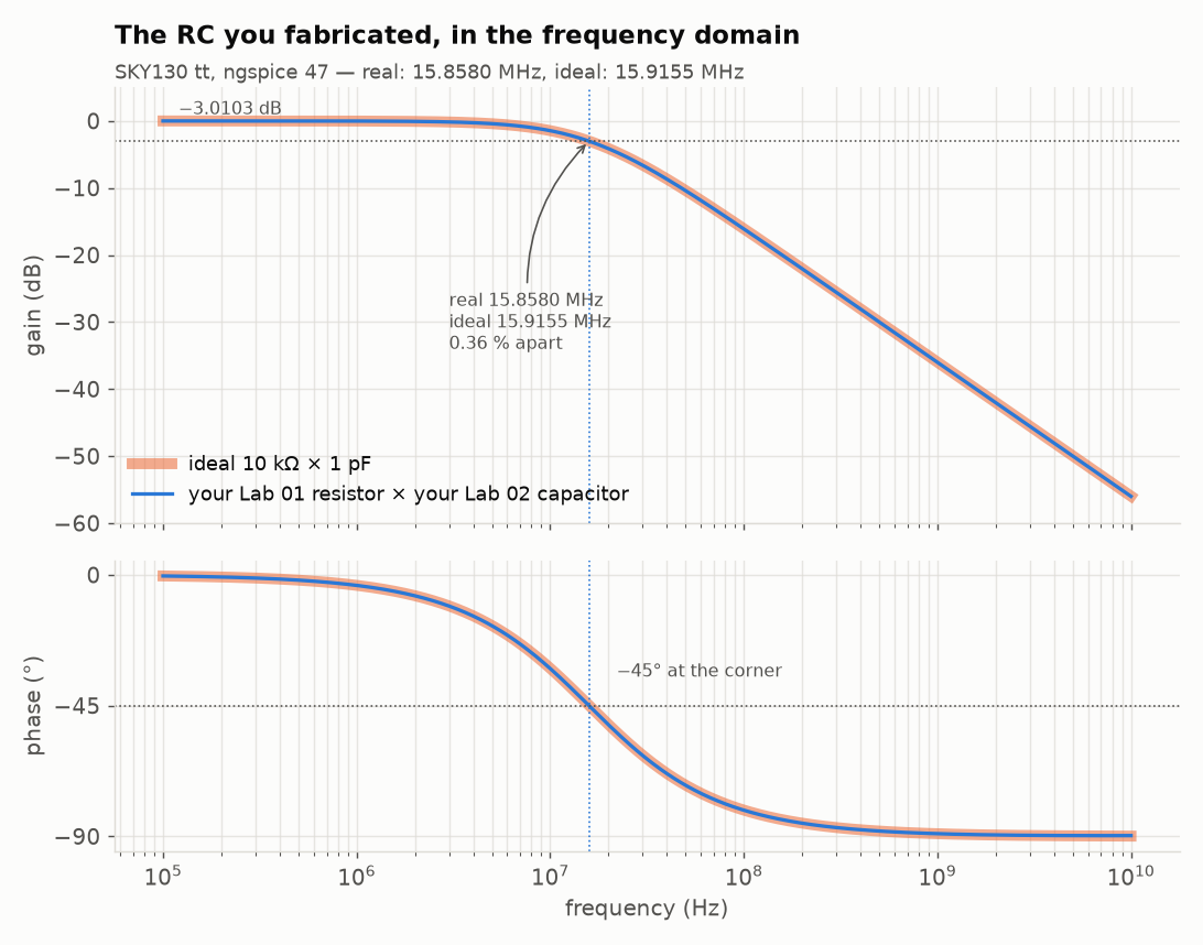
How far is your fabricated corner from the ideal one, and how far would the Part 3 design have been?
Your corner is 0.36 % from the ideal one you drew on paper, and that’s what Labs 01 and 02 (the end resistance, the perimeter capacitance, the sizing you got wrong on the first try) bought you. The same filter designed without those two labs, in Part 3, lands 5.65 % out, which is sixteen times worse.
Finishing
You’re done when make mine check, run on the resistor length and capacitor side you chose in Part 6, prints PASS -- every number matches the reference run. Your design doesn’t have to match anyone else’s; it passes when \(\tau\) is within 1 % of 20 ns and the area is under 400 µm². The “matches the reference run” part refers to the rc.spice numbers, which the checker also compares.
A transient analysis of a linear circuit has no randomness in it, so on the pinned image (ngspice-47, sky130A, tt corner) your numbers will match the ones on this page.
Question: in your Part 6 design, compare the resistor’s area with the capacitor’s. Why should they come out roughly equal?
Resistor area is roughly \(R/317.22\) µm² and capacitor area roughly \(C[\text{fF}]/2\) µm², and \(C = \tau/R\), so the total has the form \(aR + b/R\). Whenever a cost has that form, its minimum is where the two terms are the same size. The reference answer in solutions/README.md has 176.36 µm² of resistor and 164.43 µm² of capacitor, and works through why it isn’t exactly 50/50.
Once yours passes, read the same solutions/README.md. It gives one good answer, explains why the two halves of the area bill come out equal, and covers the millisecond that can’t be built.
Submit: nothing for this lab.
Going further (optional)
Part 8 isn’t in the time estimate, and nothing later in AD102 needs it. What to do next on the Course path is in the last line of this page.
Part 8 (optional): The same circuit in XSchem
So far you have typed device lines and ngspice has taken them as written. The rest of the analog track describes circuits the other way: you draw them, and the tool writes the device lines for you.
xschem/rc.sch is section E of spice/rc.spice as a drawing, with the same resistor (30.3315 µm of high-sheet poly), the same capacitor (a 22.1965 µm square of MIM) and the same pulse.
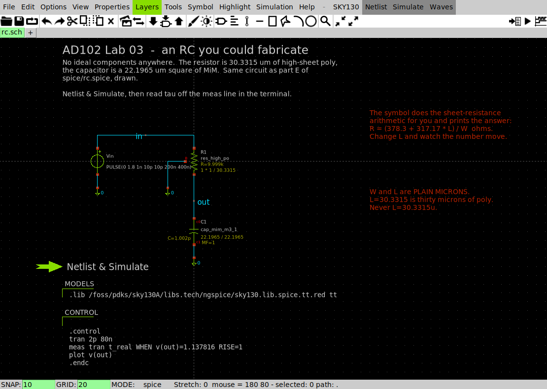
The SKY130 badge in the top right shows which parts catalogue XSchem loaded. If yours says IHP, stop and redo the PDK steps in Lab 01, Part 1. The resistor symbol prints R=9.999k beside itself, because the SKY130 symbols compute the resistance live from the W and L you give them, and the capacitor shows C=1.002p in the same way.
Turn the drawing into a netlist. You don’t need the desktop for this:
make netlist== netlisting xschem/rc.sch wrote xschem/simulation/rc.spice XR1 out in 0 sky130_fd_pr__res_high_po W=1 L=30.3315 mult=1 XC1 out 0 sky130_fd_pr__cap_mim_m3_1 W=22.1965 L=22.1965 MF=1Those are the two device lines XSchem wrote from the picture, and they’re the same two lines that section E of
spice/rc.spicehas typed by hand. A schematic is a netlist you can see.Simulate what XSchem wrote:
cd xschem/simulation && ngspice -b rc.spice; cd ../..It loads the same model library, so there’s the same wait. The output includes a warning you can ignore, which appears because the schematic asks for a plot that batch mode can’t draw:
Warning: command 'plot' is not available during batch simulation, ignored!
    You may use Gnuplot instead.
The
measstill ran, and its answer is the line below the warning.If you have the noVNC desktop up, open the schematic:
echo $PDK        # must say sky130A
make edit
XSchem opens on the drawing. Click Netlist & Simulate in the top left of the canvas, and the waveform appears in its own window.
Double-click the resistor symbol:
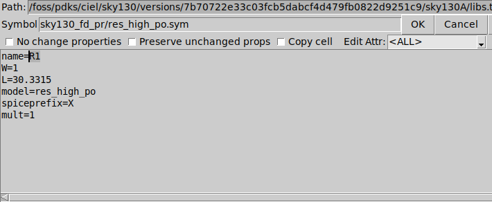
The XSchem properties dialog for R1, listing name=R1, W=1, L=30.3315, model=res_high_po, spiceprefix=X, mult=1 That’s your device line, laid out as a form. Change
L, press OK, and watch the printedR=on the symbol change. Then re-simulate and watch \(\tau\) follow it.Notice that the dialog has no units anywhere.
L=30.3315is thirty micrometres, andL=30.3315uwould be thirty millionths of a micrometre, which the schematic editor will accept just as happily as a text deck would.
You should see: after step 2,
t_real = 1.10412e-08Subtract the same 1.005 ns offset as in Part 1 and you get \(\tau = 10.0362\) ns, the same five figures as section E. The picture and the deck agree because they describe the same circuit.
AD103 is done entirely in XSchem (you’ll draw a transistor, a diode and then a CMOS inverter). Its Lab 01 starts from an empty canvas and doesn’t assume you have used XSchem before, so treat this part as a preview rather than a prerequisite.
Next on the Course path: read Process corners and Matching and Pelgrom’s law, then do Lab 04: Two resistors that disagree.