Waveforms
This page answers: the test says q is 0x32, expected 0x31. I have read the RTL four times and it looks right. Now what?
The next step is to look at the wires themselves, in a waveform. An assertion tells you that something was wrong at one instant, while a waveform shows what everything was doing for the whole run. You reach for one when the assertion has stopped narrowing things down, usually because the wrong value came from somewhere you weren’t watching, or because the value was right but arrived at the wrong time.
Most bugs in this course are quicker to find by improving the assertion message than by opening a viewer, and if you make a habit of opening the waveform first, it will cost you hours. Some bugs, though, show up only in the picture, and this page is about those. You’ll do everything it describes in cocotb on a counter, Part 5.
Getting a waveform out
Running make waves in labs/cocotb-intro runs test_04_waves.py with waveform dumping turned on, and prints this:
    11.00ns INFO  cocotb.counter  reset released at t = 11 ns
   111.00ns INFO  cocotb.counter  counted to 0x0A at t = 111 ns
   121.00ns INFO  cocotb.counter  loaded 0xFF at t = 121 ns  <-- zoom here
   151.00ns INFO  cocotb.counter  held 3 clocks with en low, still 0xFF, t = 151 ns
   152.00ns INFO  cocotb.counter  en high again at t = 152 ns; the wrap is the next edge
   161.00ns INFO  cocotb.counter  wrapped to 0x00 at t = 161 ns
   211.00ns INFO  cocotb.counter  finished at t = 211 ns with q = 0x05
...
FST info: dumpfile /work/labs/cocotb-intro/build/waves/counter.fst opened for output.

   wrote  /work/labs/cocotb-intro/counter.fst   (699 bytes)
   wrote  /work/labs/cocotb-intro/counter.vcd   (1098 bytes)
The FST info: dumpfile ... opened for output. line appears after the results table because it comes from Icarus closing the file at the end of the run. It isn’t an error, and by the time it’s printed the test has already passed.
All of this comes from one make variable, WAVES=1, passed to cocotb’s makefile. With it set, cocotb’s Icarus makefile generates a dump module for you and adds it to the compile, so you never have to write $dumpfile or $dumpvars yourself:
/foss/tools/bin/iverilog ... -s cocotb_iverilog_dump rtl/counter.sv build/waves/cocotb_iverilog_dump.vThe dump is written to $(SIM_BUILD)/$(COCOTB_TOPLEVEL).fst, which here is build/waves/counter.fst. The package’s make waves then copies it up to counter.fst and converts it with fst2vcd, so you end up with both formats.
If you drive
sim.mkby hand and changeRTL=, changeSIM_BUILD=along with it. cocotb’s makefile relinks only when the sources are newer thansim_build/sim.vvp, so a second run against a different design can quietly rerun the first one. The test goes green, but it has tested something other than what you meant, and that’s why every package target passes its ownSIM_BUILD.
If you search for “cocotb waveform” you’ll find
COCOTB_PLUSARGS=+WAVESand hand-written$dumpvarstestbench shells, and both are real techniques. SimProc’stb.vuses the$dumpvarsapproach, because it already has a Verilog shell to put it in. For a design that cocotb attaches to directly,WAVES=1does the same job with one variable, so write the shell yourself only when you need to dump a subset of a large design.
FST or VCD
The two formats hold the same information in different encodings. Use FST unless some tool refuses to read it.
| This counter | SimProc, labs/common → make waves |
|
|---|---|---|
| Signals in the file | 7 | 190 (across 11 scopes) |
| VCD | 1,098 bytes | 3,007,592 bytes |
| FST | 699 bytes | 12,152 bytes |
As FST, the SimProc dump is 247 times smaller. VCD is plain text, with every value change written out in ASCII, while FST is compressed and indexed, so a viewer can seek to any point in it without reading the whole file. fst2vcd and vcd2fst, both on the workbench PATH, convert in either direction.
VCD is still worth knowing, because everything reads it, and because when you suspect the viewer rather than the data you can open a VCD file with less and look at it directly.
Opening a viewer
Start Surfer and GTKWave by typing their names in a terminal on the noVNC desktop, never by clicking a desktop icon. Both viewers print their real complaints to the terminal they were started from. If you start one from a menu there is no such terminal, so a viewer that can’t open your file tells you nothing and just sits there looking normal.
Surfer
The workbench has Surfer 0.6.0. Here is counter.fst open in it:

That’s the whole 211 ns run. Reset releases, the counter walks from 00 to 0a, load pulses and d puts ff in, and en drops for three clocks while q sits at ff. Then en comes back, tc goes high for exactly one clock, and the count wraps to 00.
Using it takes three steps:
- In the Scopes pane, top left, click the module (
counter). For SimProc you walk downtb→tt_um_ieeeuoftasic_simproc→U1→CPU1. - In the Variables pane, bottom left, click signals to add them, or type
module_add counterin the command box to add every signal in a scope at once. - Drag on the time ruler to zoom.
Ctrl+ scroll also zooms.
The time axis is in picoseconds, because cocotb’s default simulation precision is 1 ps. That’s why the ruler in the screenshot reads
20000 ps,40000 psand so on, and20000 psis 20 ns. Your test logs times in nanoseconds, so multiply them by 1000 before you go looking for them on the ruler.
Surfer can also read a command file, which saves you re-adding the same signals every time. We made the screenshot that way, with a file containing module_add counter passed to Surfer with surfer -c.
GTKWave
GTKWave (v4.0.0-prealpha on the workbench) is the older of the two. It reads both formats, and prints FSTLOAD | Processing 7 facs. / Built 7 signals and 0 aliases. when it loads FST and [0] start time. / [211000] end time. when it loads VCD.
GTKWave has one trap that you should know about before you run into it, which is that it opens fully zoomed in, at time zero:
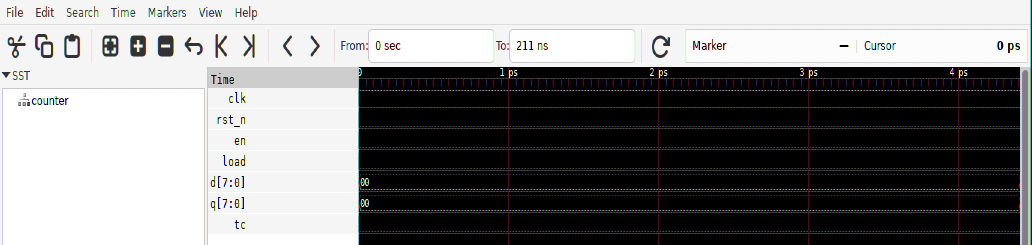
The waveform loaded correctly: the header even says To: 211 ns, and the seven signals are listed on the left. The wave pane looks empty because it’s showing only the first four picoseconds of the 211 ns run, before anything has happened. The first clock edge after t = 0 is at 10 ns, which is 2,500 screens to the right.
The fix is Zoom Fit, which is under View → Zoom → Zoom Best Fit, on Ctrl Alt F, and on the toolbar as the magnifier with the square in it. Do it first, every time you open a file, before you conclude anything from what’s on the screen.
If GTKWave opens with an empty signal list instead, that’s the other half of the same trap. The signals are in the SST tree at the top left, and nothing appears in the wave pane until you Append them to it. A .gtkw save file remembers that choice, so you only have to make it once. counter.gtkw ships with the package, and it’s just a plain-text list of signal names.
Use Surfer unless you have a reason to prefer GTKWave: Surfer opens at a sensible zoom, its keyboard handling is better, and it’s useful without a save file. GTKWave is the one to use when you want its analogue rendering or transaction filters, or when you’re following someone else’s .gtkw.
What to look at first
A whole processor has a lot of signals (SimProc’s dump has 190), and if you add all of them you’ll spend your time scrolling instead of debugging. Start with these four kinds of signal, in this order.
- The clock and the reset. They aren’t interesting in themselves, but when everything is wrong, they’re usually the first thing that went wrong. A clock that never toggles means you forgot
cocotb.start_soon, and a reset that never releases means you droverst_nand never raised it. Either one gives you a screen of flat lines, and either takes seconds to fix. - Anything
Xor red. In both Surfer and GTKWave, red means an undriven or conflicting signal. AnXpropagates (one undriven input turns a whole datapath red three cycles later), so trace it back to the first signal that is red and fix that one, because everything downstream of it is only a symptom. - The state register. In a design with a control FSM, it carries more information than any other signal. In SimProc it’s
CPU1.curr_state, which decodes toIDLEandCYCLE_1toCYCLE_5. If you watch it walkCYCLE_1 → CYCLE_2 → CYCLE_3 → CYCLE_1, you know that a three-cycle instruction retired, before you’ve looked at any data. - Whatever your assertion named, at the time it named. That’s why
test_04_waves.pylogsloaded 0xFF at t = 121 ns <-- zoom here. If you know the timestamp before you open the viewer, you can go straight to it and read the waveform there, instead of scrolling through the whole run looking for the problem.
Before you add a fifth signal, ask yourself what you expect it to show. If you can’t say, you’re browsing rather than debugging, and you’d do better to go back to the assertion and make it print more.
A bug you can only see in the picture
Run against the broken counter (rtl/counter_broken.sv, the same file with en & deleted from tc), test_04_waves still passes, and its log is identical line for line to the good run’s, with the same times, the same values and the same PASS. That’s because test_04_waves never checks tc, so nothing in the text output can tell the two counters apart. In the waveform the difference is easy to see:

Compare the bottom trace with the earlier screenshot. On the good counter, tc is one narrow pulse, one clock wide, at t = 152–161 ns: the one clock where q is 0xFF and en is high. On the broken counter, tc goes high at t = 121 ns, the instant q becomes 0xFF, and stays high for the whole four-clock stretch, including the three clocks where the counter isn’t moving.
Everything else on the screen is pixel-identical, so the only difference between the two runs is one trace that is four times too wide, and the log doesn’t show it at all. Some bugs have the shape of a waveform, and recognising those shapes is the reason to learn the viewer before you need it rather than during the hour you need it.
Check yourself
- GTKWave shows seven flat signals and the header says
To: 211 ns. What do you do first? - You open a SimProc waveform to chase a wrong register value. Which signals do you add, in what order?
Next: cocotb on a counter.