Lab 02: Harmonic builder
You’ll add sines together into a chord, build a square wave out of odd harmonics while its spectrum updates beside it, and watch the duty cycle of a pulse train switch even harmonics on and off. Before the scripts run, you’ll work out the harmonic amplitudes and frequencies they should show.
Lab package: labs/lab-02-harmonic-builder/
Before you start
Finish Lab 01.
Read Movement II: Adding signals, Timbre and harmonics and Rhythm and duty cycle.
In a terminal in the noVNC desktop, go to the lab folder:
. /foss/designs/common/.designinit
mod ad101
cd labs/lab-02-harmonic-builder
Time: about 1 hour.
As in Lab 01, Part 1 is a snippet on its own, and the other parts each pair an explorer (python3 src/explore.py --figure <id>) with a snippet. You save each snippet as a new .py file in this folder and run it with python3 <file>.py.
Part 1: Build a chord
What does the sum of three notes look like in time?
Save this as
chord.pyand run it. It adds the three notes of a C-major triad, sample by sample:import numpy as np import matplotlib.pyplot as plt fs = 10_000 t = np.arange(0, 0.02, 1 / fs) # a C-major triad: C4, E4, G4 (Hz) c = np.sin(2 * np.pi * 261.6 * t) e = np.sin(2 * np.pi * 329.6 * t) g = np.sin(2 * np.pi * 392.0 * t) chord = c + e + g fig, axes = plt.subplots(2, 1, sharex=True, figsize=(7, 5)) axes[0].plot(t * 1e3, c, label="C4", alpha=0.7) axes[0].plot(t * 1e3, e, label="E4", alpha=0.7) axes[0].plot(t * 1e3, g, label="G4", alpha=0.7) axes[0].legend(fontsize=8) axes[0].set_ylabel("three notes") axes[1].plot(t * 1e3, chord, color="black") axes[1].set_ylabel("sum (the chord)") axes[1].set_xlabel("Time (ms)") plt.tight_layout() plt.show()
You should see the three notes in the top panel and their sum in black in the bottom panel. From the bottom trace alone you couldn’t tell by eye that it’s made of three sines, and Movement III gives you a tool that can.
Part 2: Build a square wave from sines (F4/F5)
Which sines, at which amplitudes, add up to a square wave?
Open the Fourier assembler, which shows F4 (the waveform) and F5 (its spectrum) in the same window:
python3 src/explore.py --figure f4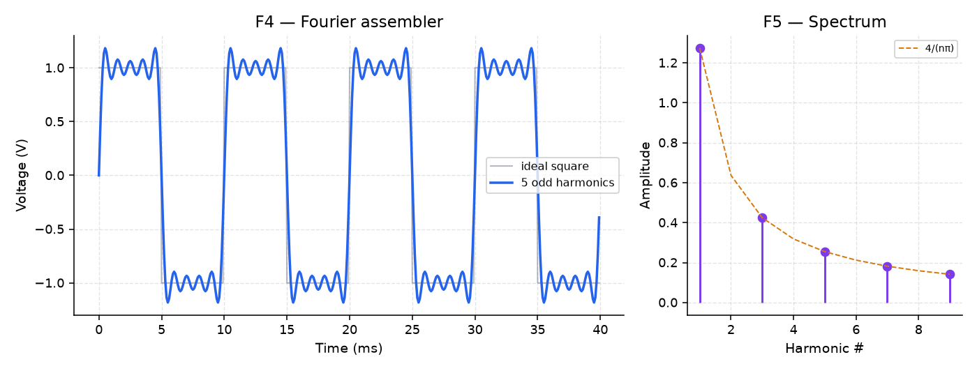
F4/F5 All five harmonics (n=1, 3, 5, 7, 9) start ticked, with their amplitudes set to \(4/(n\pi)\) rounded to the sliders’ 0.02 steps, which is why A1 reads 1.28. Untick 3, 5, 7 and 9 so that only n=1 is left.
You should see a plain sine in F4 and a single stem in F5.
Next you’ll tick 3, 5, 7 and 9 back on, one at a time. Before you do, predict whether the overshoot at the square’s edges will shrink away as you add harmonics, and write your answer down. Then tick them on.
You should see the sum walk toward the gray ideal square, with an overshoot near each edge that doesn’t go away. The F5 stems update in step with the waveform and sit on the dashed \(4/(n\pi)\) curve, the square-wave recipe from Timbre and harmonics.
Why doesn’t the overshoot go away as you add harmonics?
TipAnswerThe overshoot is called Gibbs ringing. It comes from approximating a sharp edge with a finite number of sines, so it stays however many harmonics you add. A real digital clock on an oscilloscope shows the same shape.
Drag the amplitude sliders (A1 to A9) toward and away from \(4/(n\pi)\).
You should see the sum stop looking like a square as the stems move off the dashed curve, and look like one again as they move back onto it. Close the window.
Save this as
square_from_sines.py, but don’t run it yet. It prints the amplitude it uses for each harmonic:import numpy as np import matplotlib.pyplot as plt fs = 10_000 t = np.arange(0, 0.02, 1 / fs) f0 = 200.0 # fundamental frequency, Hz harmonics = [1, 3, 5, 7, 9] # odd harmonics only built = np.zeros_like(t) for n in harmonics: amplitude = 4 / (n * np.pi) # the square-wave recipe built += amplitude * np.sin(2 * np.pi * n * f0 * t) print(f"n = {n} amplitude = {amplitude:.3f}") ideal_square = np.sign(np.sin(2 * np.pi * f0 * t)) plt.plot(t * 1e3, ideal_square, color="gray", linestyle="--", label="ideal square") plt.plot(t * 1e3, built, label=f"sum of {len(harmonics)} harmonics") plt.xlabel("Time (ms)") plt.ylabel("Voltage (V)") plt.legend() plt.show()The
4 / (n * np.pi)line is the recipe from the square-wave formula in Timbre and harmonics. Before you run it, work out \(4/(n\pi)\) for n = 1, 3, 5, 7 and 9 to three decimal places, and write the five numbers down. Then run it.You should see:
n = 1   amplitude = 1.273
n = 3   amplitude = 0.424
n = 5   amplitude = 0.255
n = 7   amplitude = 0.182
n = 9   amplitude = 0.141
These are the values the F4 sliders showed, before they were rounded to 0.02. The plot shows the sum of five harmonics close to the dashed square, with ringing at the edges.
Change the list to
harmonics = [1]and re-run. Then add3, then5,7and9, re-running each time.You should see the sum start as a plain sine and walk toward the dashed square with each sine you add, and one more
amplitudeline printed each time. The overshoot right at the edges appears and stays, as it did on F4. That’s the Gibbs ringing from step 3, not a bug in your code.
Part 3: Duty cycle and even harmonics (F6)
Which harmonics does a pulse train’s duty cycle switch on and off?
Open the duty-cycle explorer:
python3 src/explore.py --figure f6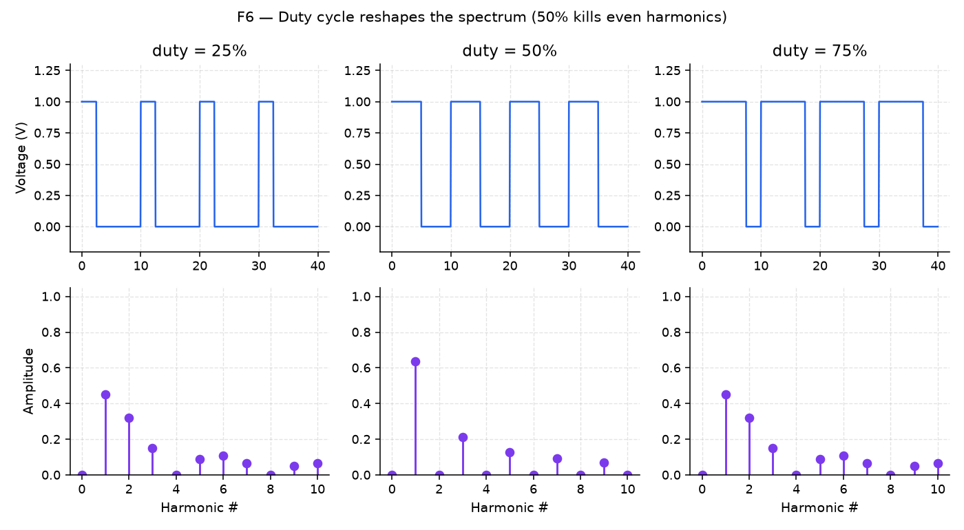
F6 It starts at 50% duty, and the box under the plots reads
duty = 50% → even harmonics GONE (50% duty).Sweep Duty from 25% to 50% to 75% and watch the even-numbered stems in the spectrum.
You should see the even stems vanish at exactly 50% and come back on either side of it (harmonic 2 is the easiest to spot), with the box switching to
even harmonics PRESENT. Close the window.Save this as
duty_sweep.py, but don’t run it yet. It usesnp.fft.rfft, the “count the harmonics for me” machine you’ll meet properly in The FFT as an equalizer. For now, treat it as a black box:import numpy as np import matplotlib.pyplot as plt fs = 10_000 t = np.arange(0, 0.05, 1 / fs) f0 = 200.0 fig, axes = plt.subplots(1, 3, figsize=(10, 3), sharey=True) for ax, duty in zip(axes, [0.25, 0.50, 0.75]): phase = (f0 * t) % 1.0 pulse = np.where(phase < duty, 1.0, 0.0) spectrum = np.abs(np.fft.rfft(pulse - pulse.mean())) freqs = np.fft.rfftfreq(len(pulse), d=1 / fs) ax.stem(freqs[:100], spectrum[:100]) ax.set_title(f"duty = {duty:.0%}") ax.set_xlabel("Frequency (Hz)") plt.tight_layout() plt.show()It plots the spectra of 200 Hz pulse trains at 25%, 50% and 75% duty. Before you run it, write down the frequencies between 0 and 2000 Hz where you expect stems in the 50% panel. Then run it.
You should see three stem plots from 0 to 2000 Hz. In the middle panel (50%) the only stems are at odd multiples of 200 Hz: 200, 600, 1000, 1400 and 1800 Hz. The 25% and 75% panels also have stems at even multiples, such as 400 Hz.
Finishing
You’re done when the five amplitudes you worked out match what square_from_sines.py prints (Part 2, step 5), and the stems in the 50% panel of duty_sweep.py sit at the frequencies you wrote down (Part 3, step 3).
Questions
- Why doesn’t adding more harmonics remove the overshoot at a square’s edges? (Answered in Part 2, step 3.)
Submit
Nothing to submit.
Next on the Course path: read Movement III, The FFT as an equalizer, Finding a quiet note, Distortion and THD and Sampling fast enough, then do Lab 03: Spectrum detective.