Lab 03: Spectrum detective
In this lab you’ll compute your first FFT and match test signals to their spectra. Then you’ll find a tone hidden under noise and confirm it with a checker, watch clipping create harmonics and read off the THD, and make a tone lie about its frequency by sampling it too slowly. Along the way you’ll predict three numbers before a script prints them: a dB gap, a THD and an alias frequency.
Lab package: labs/lab-03-spectrum-detective/
Before you start
Finish Lab 02.
Read Movement III: The FFT as an equalizer, Finding a quiet note, Distortion and THD and Sampling fast enough.
Know the dB table in Reading plots.
In a terminal in the noVNC desktop, go to the lab folder:
. /foss/designs/common/.designinit
mod ad101
cd labs/lab-03-spectrum-detective
Time: about 1.5 hours, not counting the optional Part 5.
As before, most parts pair an explorer (python3 src/explore.py --figure <id>) with a short snippet that you save as a new .py file in this folder and run with python3 <file>.py.
Part 1: Your first FFT (F7)
How does the same signal look in time and in frequency?
Save this as
first_fft.py, but don’t run it yet. It builds a two-note chord, A4 and E5, and plots it in time and in frequency:import numpy as np import matplotlib.pyplot as plt fs = 10_000 t = np.arange(0, 0.2, 1 / fs) # a longer window gives a sharper spectrum # a two-note chord: A4 and E5 v = np.sin(2 * np.pi * 440 * t) + 0.5 * np.sin(2 * np.pi * 659 * t) spectrum = np.abs(np.fft.rfft(v - v.mean())) freqs = np.fft.rfftfreq(len(v), d=1 / fs) spectrum_db = 20 * np.log10(np.maximum(spectrum, 1e-6)) fig, axes = plt.subplots(2, 1, figsize=(7, 6)) axes[0].plot(t * 1e3, v) axes[0].set_xlabel("Time (ms)") axes[0].set_ylabel("Voltage (V)") axes[0].set_title("time domain") axes[1].plot(freqs, spectrum_db) axes[1].set_xlim(0, 1000) axes[1].set_xlabel("Frequency (Hz)") axes[1].set_ylabel("Magnitude (dB)") axes[1].set_title("frequency domain") plt.tight_layout() plt.show()In the script,
v - v.mean()removes any DC offset before the FFT, andnp.maximum(..., 1e-6)makes surelog10is never handed a zero.E5 has half A4’s amplitude. Before you run it, use the dB table in Reading plots to predict how many dB below the A4 peak the E5 peak will sit, and write it down. Then run it.
You should see a tangle of two overlapping wiggles in the top plot and two clear peaks in the bottom one: A4 at 440 Hz and E5 near 659 Hz, which sit at 60.0 dB and 53.4 dB in the course image. The dB values are raw FFT magnitudes, so the peaks sit far above 0 dB, and only the gap between them means anything. Close the window.
How big is the gap, and why isn’t it exactly the 6 dB the table gives?
TipAnswerA ratio of ×0.5 is about −6 dB, so E5 should sit about 6 dB below A4. The plot shows 60.0 − 53.4 = 6.6 dB. The extra 0.6 dB comes from leakage, which Finding a quiet note describes and the optional Part 5 shows you on F10. In the 0.2 s window, 440 Hz fits a whole number of cycles (88) but 659 Hz doesn’t (131.8), so part of the E5 peak smears into the neighbouring bins and the peak itself comes out lower. If you change
659to660in the script, the gap comes out at 6.0 dB.Open the twin-panel explorer:
python3 src/explore.py --figure f7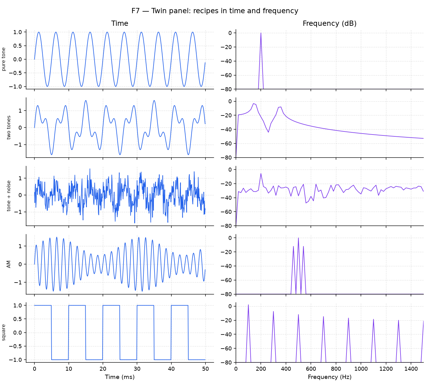
F7 Click through the signals on the left: pure tone, two tones, tone + noise, AM and square. AM (amplitude modulation) is a 500 Hz tone, called the carrier, whose loudness wobbles up and down at 40 Hz. Then switch the “dB scale” and “log freq” boxes on and off.
You should see one spike for the pure tone, two spikes for two tones, a carrier with a sideband on each side for AM, and a comb of odd harmonics for the square. With dB on, you can also see small peaks that the linear axis hides. Close the window.
Part 3: Distortion and THD (F9)
How much new energy does clipping put into the harmonics?
Open the distortion explorer:
python3 src/explore.py --figure f9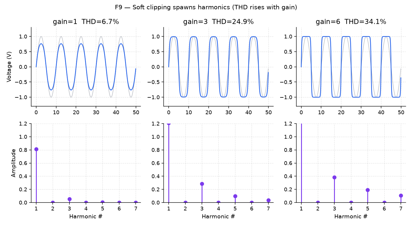
F9 Raise “Gain (into tanh)” and watch the waveform, the harmonic stems and the THD readout. \(\tanh\) is the smooth clipping curve from Distortion and THD, and more gain drives the sine further into it.
You should see the soft clipping flatten the peaks of the sine, the odd harmonics grow, and the THD climb from about 2% at the lowest gain (0.5) to about 35% at gain 6. Set the gain to 1 and write down the THD it reads. Close the window.
Save this as
clip_thd.py, but don’t run it yet. It clips a sine at three gains, 1, 3 and 8, and measures the THD from the spectrum. It only prints its results, so no plot window opens:import numpy as np import matplotlib.pyplot as plt fs = 10_000 t = np.arange(0, 0.1, 1 / fs) f0 = 200.0 clean = np.sin(2 * np.pi * f0 * t) for gain in (1.0, 3.0, 8.0): distorted = np.tanh(gain * clean) # soft clip — bigger gain = harder clip spectrum = np.abs(np.fft.rfft(distorted - distorted.mean())) freqs = np.fft.rfftfreq(len(distorted), d=1 / fs) def amp_at(f_hz): return spectrum[np.argmin(np.abs(freqs - f_hz))] a1 = amp_at(f0) harmonics_power = sum(amp_at(f0 * n) ** 2 for n in (2, 3, 4, 5)) thd = (harmonics_power ** 0.5) / a1 print(f"gain={gain:>4.1f} THD = {thd*100:5.1f}%")Before you run it, use your F9 reading to predict the THD it will print at gain 1, and decide whether gain 3 and gain 8 will print more or less. Write your predictions down, then run it.
You should see:
gain= 1.0   THD =   6.7%
gain= 3.0   THD =  24.9%
gain= 8.0   THD =  36.0%
F9 at gain 1 reads
THD = 6.7%, the same as the script. The two don’t measure quite the same thing, though: the script sums harmonics 2 to 5 while F9 sums harmonics 2 to 7, so they can differ slightly at high gain.
Part 4: Sampling and aliasing (F11)
How slowly can you sample a tone before it shows up at the wrong frequency, and which frequency does it show up at?
Open the aliasing explorer:
python3 src/explore.py --figure f11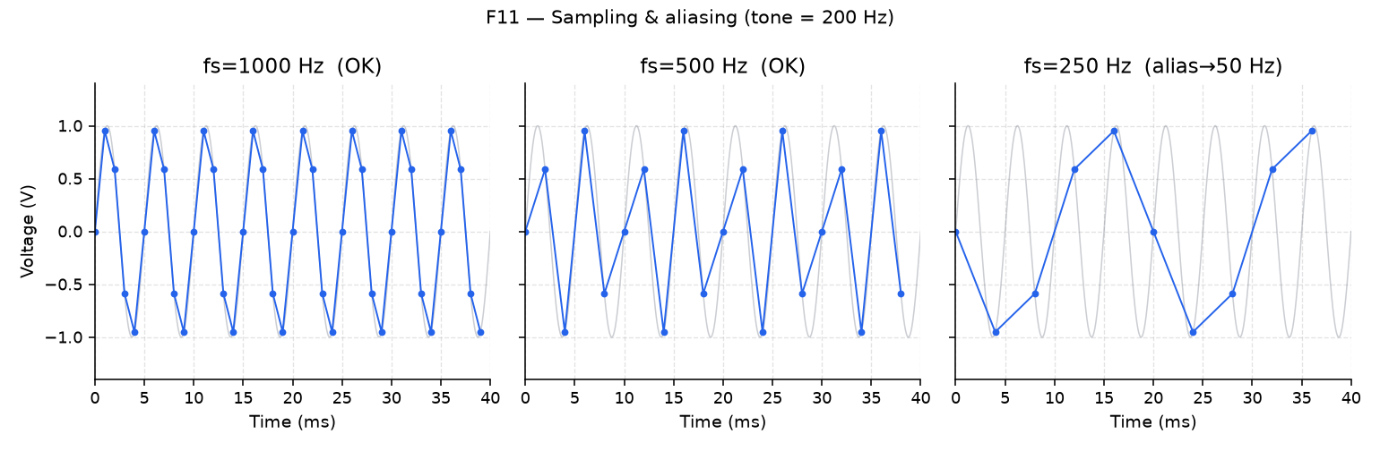
F11 The tone is 200 Hz and the sample rate starts at 1000 Hz, so the box at the bottom ends in
OK (fs > 2f). TheNyquistvalue in that box is half the sample rate.Before you move anything, work out the sample rate below which a 200 Hz tone aliases, and write it down.
Drag “Sample rate (Hz)” down slowly until the box changes, then set it to 250 Hz.
You should see the box switch to
ALIASED → appears as … Hzonce the sample rate drops below 400 Hz, a bogus slow sine appear over the samples, and the spectrum peak fold below Nyquist. At 250 Hz the box readsALIASED → appears as 50 Hz. Close the window.Save this as
aliasing.py, but don’t run it yet. It samples a 900 Hz tone twice, once above Nyquist and once below. In this script “Nyquist” means the Nyquist rate, \(2f\) = 1800 Hz, rather than F11’sNyquistvalue of \(f_s/2\), and Sampling fast enough explains the difference between the two:import numpy as np import matplotlib.pyplot as plt true_freq = 900.0 # Hz — the real tone duration = 0.02 for fs in (5000.0, 1000.0): # first well above Nyquist, then below it t = np.arange(0, duration, 1 / fs) v = np.sin(2 * np.pi * true_freq * t) nyquist_ok = fs > 2 * true_freq label = "OK — above Nyquist" if nyquist_ok else "ALIASED — below Nyquist" plt.plot(t * 1e3, v, marker="o", label=f"fs={fs:.0f} Hz ({label})") plt.xlabel("Time (ms)") plt.ylabel("Voltage (V)") plt.legend(fontsize=8) plt.title(f"true tone = {true_freq:.0f} Hz") plt.show()In step 3, at 250 Hz, F11 showed the 200 Hz tone as 50 Hz, which is 250 − 200. That’s a general rule: a tone that lies between half the sample rate and the sample rate shows up at the sample rate minus the tone’s frequency. Use it to predict the frequency the
fs=1000points will appear to have, and write it down. Then run the script.
You should see the fs=5000 points trace a recognizable 900 Hz wiggle, while the fs=1000 points join into a slow, wrong-looking wave with a period of about 10 ms (100 Hz, which is 1000 − 900), like the backwards-spinning wheel in Sampling fast enough.
Part 5 (optional): Spectral leakage (F10)
What happens to a peak when the window doesn’t hold a whole number of cycles, and what does a Hann window do about it? Nothing in Parts 1 to 4 depends on this part, and it isn’t in the time estimate.
Open the leakage explorer:
python3 src/explore.py --figure f10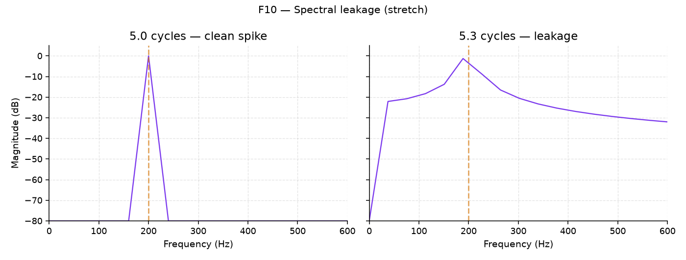
F10 Set “Cycles in window” to 5.0, then to 5.3.
You should see a clean spike at 5.0 (the label reads
clean spike (integer cycles)) and a smeared peak at 5.3 (smeared peak (leakage!)).Leave it at 5.3 and tick “Hann window”.
You should see the skirts (the smeared energy on either side of the peak) drop. Close the window.
Why do spectra measured on a real bench look soft instead of like textbook sticks?
TipAnswerIt’s leakage. A real measurement window doesn’t hold a whole number of cycles of every tone in the signal, so the peaks smear sideways into their neighbouring frequency bins, just as they did at 5.3 cycles here. A window function such as Hann tapers the start and end of the recorded segment toward zero, which reduces the smear.
Finishing
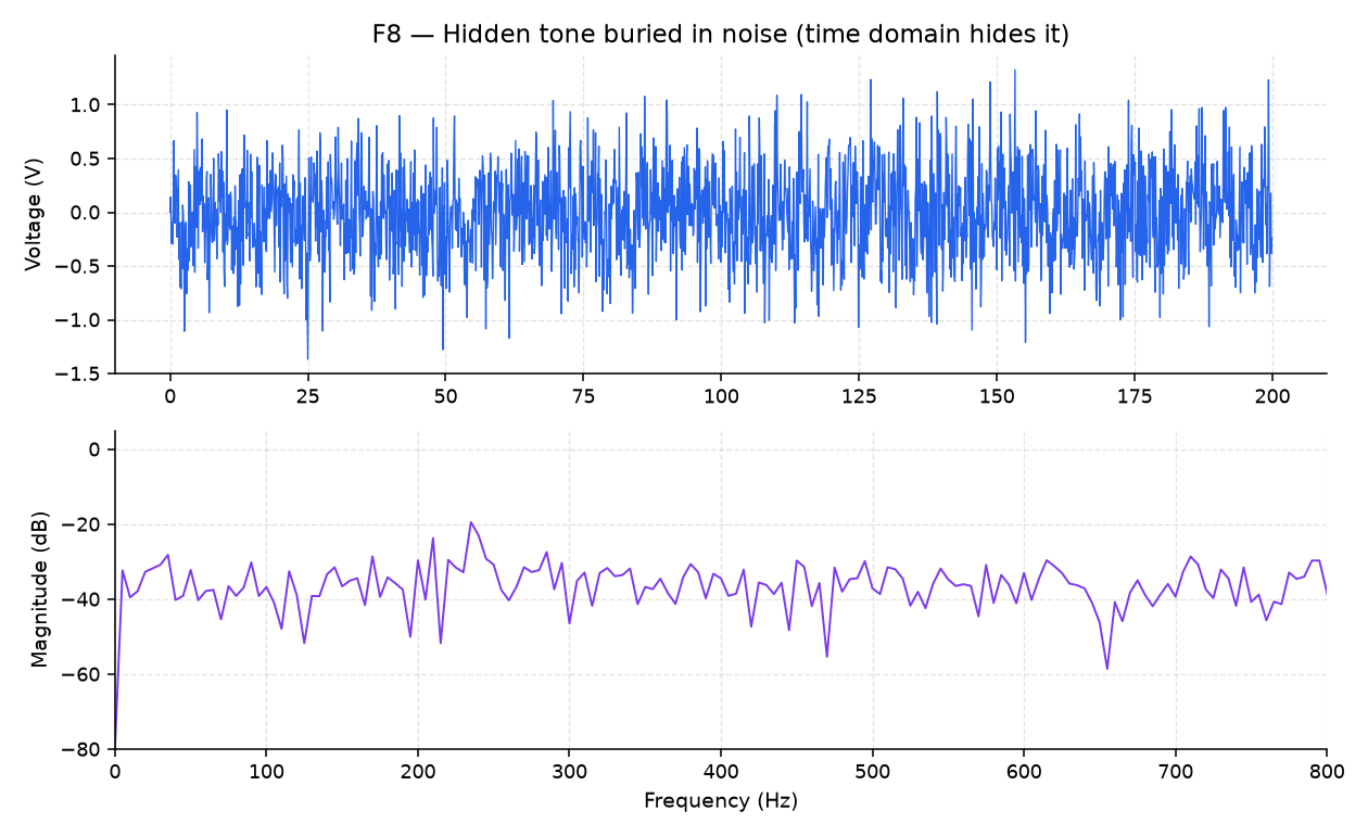
You’re done when python3 src/check.py --guess <Hz>, with the frequency you read off F8 yourself, prints Correct! (Part 2, step 3), and your predictions from Parts 1, 3 and 4 are written down next to what the scripts printed.
Questions
- Why is the E5 peak 6.6 dB below A4 and not 6.0 dB? (Answered in Part 1, step 1.)
- Below what sample rate does a 200 Hz tone alias? (Answered in Part 4, steps 2 and 3.)
Submit
Nothing to submit.
Next on the Course path: read Movement IV, Filters are tone knobs, Reading a Bode plot, Filtering a beat and More filter shapes, then do Lab 04: RC filter and Bode.