The operating point
When you can’t use superposition on a circuit and you can’t solve its equation by hand either, the only way left to get a number out of it is to search for one. You can run that search yourself on paper in about ninety seconds, and it’s worth doing once, because it’s what every SPICE simulation you launch is doing underneath.
A resistor and a diode in series
The circuit has one supply, one resistor and one diode:
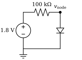
There is only one unknown, v_node, and KCL at that node gives you one equation for it: the current flowing down through the resistor has to equal the current through the diode.
\[ \frac{1.8 - v}{100\,\text{k}\Omega} \;=\; I_{\text{diode}}(v) \]
The left side is a straight line in \(v\). The right side is the diode’s curve, which the next page shows is an exponential in \(v\), so written out in full the equation is
\[ \frac{1.8 - v}{100\,000} \;=\; I_0\!\left(e^{v/nV_T} - 1\right) \]
with \(v\) appearing both outside an exponential and inside one. No rearrangement of this equation leaves \(v\) alone on one side. That’s a property of the equation itself, whatever algebra you try, and mathematicians call an equation like this transcendental. The usual way to deal with one is to stop trying for an exact answer and get close to it instead, then closer still.
Load lines
Plot the diode’s curve, and then plot the resistor’s equation on the same axes. The resistor’s equation, \(i = (1.8 - v)/R\), is a straight line with an intercept of \(1.8/R\) and a slope of \(-1/R\). It’s called the load line, and drawing one is still the fastest way to see what a circuit like this will do.
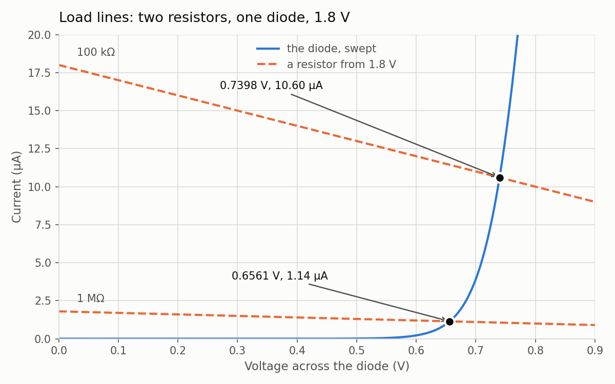
Produced by src/plot_iv.py in the Lab 02 package. The blue curve is plotted from the same 1901 rows as every other diode plot in this course.
Every point on the blue curve satisfies the diode’s equation, and every point on an orange line satisfies the resistor and the supply. The only point that satisfies all of them at once is where the two cross, and that crossing, a single voltage and current together, is the operating point.
Two things follow from the picture:
- Changing the resistor moves the operating point along the diode’s curve; it can’t move off it. Going from 1 MΩ to 100 kΩ multiplies the current by 9.27 but moves the voltage by only 83.7 mV, so you get roughly ten times the current for less than a tenth of a volt.
- The diode’s curve is so steep near 0.7 V that even a large change in the load line produces only a small change in voltage. That’s where the rule of thumb “a diode drops 0.7 V” comes from, and Three diode models puts a number on how good a rule it is.
Worked example: guess, correct, repeat
You can also find the operating point numerically, with a calculator and two facts taken from the measured curve. Start from the rule of thumb, 0.7 V, and use one measured anchor point: the diode carries 3.917437 µA at 0.700 V, and its current rises by one decade for every 77.04 mV.
- Guess \(v = 0.700\) V. The resistor then delivers \((1.8 - 0.700)/100\,\text{k}\Omega = 11.000\ \mu\text{A}\).
- Correct. A diode carrying 11.000 µA wouldn’t sit at 0.700 V; it would sit at \(0.700 + 0.07704\log_{10}(11.000/3.917437) = 0.7345\) V.
- Repeat. At 0.7345 V the resistor delivers only 10.655 µA, which the diode holds at 0.7335 V. That voltage gives 10.665 µA, and 10.665 µA gives 0.7335 V again, so the answer has stopped moving.
After three rounds of arithmetic, the hand answer is 0.7335 V and 10.665 µA.
What ngspice gets
ngspice’s operating-point analysis, op, solves the same circuit, and it too works by iterating until the answer stops moving. For three values of the resistor it gives:
| \(R\) | diode voltage | current |
|---|---|---|
| 10 kΩ | 0.8905358 V | 90.94642 µA |
| 100 kΩ | 0.7398473 V | 10.60153 µA |
| 1 MΩ | 0.6561163 V | 1.143884 µA |
Your hand answer of 0.7335 V and 10.665 µA was 6.3 mV and 0.60 % away from the 100 kΩ row, and you got that close with three lines of arithmetic and one measured anchor point.
The 0.60 % error comes from a real property of the device rather than from your arithmetic. You used a constant 77.04 mV per decade, but above about 0.7 V the diode’s curve has already started to bend away from that straight line. Lab 02 measures where the bend starts, 0.699 V, and the next page explains why it happens. If you redo the three steps with 86 mV per decade instead, which is the local value measured in that region, you land on 0.7373 V and 10.627 µA. That’s 2.6 mV and 0.24 % out, less than half the error.
Two independent calculations
op and a DC sweep (.dc) are different computations. op solves the nonlinear circuit once, by iterating. The diode sweep is 1901 separate solves of a different circuit, a lone diode driven by a voltage source with no resistor at all. The only reason the two should agree is that they describe the same device.
That gives you a way to check one against the other. In the sweep data, find the voltage at which the diode’s current equals the current on the 100 kΩ load line. Interpolating between the two sweep rows on either side of the crossing gives 0.739846 V and 1.060154e-05 A, and op said 7.398473e-01 V and 1.060153e-05 A. The two calculations share nothing but the device model, and they agree to six digits. When two independent routes to a number agree that closely, you can be confident the number isn’t an artifact of either route. You’ll make this comparison yourself in Lab 02, Part 5.
Every amplifier, current mirror and logic gate is designed by first choosing an operating point and then arranging for the circuit to sit at it. The back half of this course (transconductance, the CMOS inverter, the current mirror) is about picking that point on purpose, rather than discovering where the circuit ended up afterwards.
Small-signal resistance
If you zoom in far enough on any smooth curve, it looks like a straight line. Near the 1 MΩ operating point, the diode’s own sweep gives \(\Delta V = 2\) mV between the rows at 0.655 V and 0.657 V, and \(\Delta I = 65.98\) nA across the same two rows, so \(\Delta V/\Delta I\) is 30.3 kΩ. That’s the slope of \(V\) against \(I\), the reciprocal of the slope you see on the plot above, where current is drawn against voltage. A small wiggle riding on that operating point sees the diode as a 30.3 kΩ resistor, which means superposition works again, at least for the wiggle.
That is the idea behind every analog circuit you have used: the circuit is nonlinear enough to set a bias point, and everything small that happens near that point is treated as linear. If you move the operating point, the resistance moves with it. At the 100 kΩ point the same measurement gives 4.12 kΩ, about seven times smaller, while the current there is 9.27 times larger.
For a pure junction those two ratios would be the same. Differentiating the diode equation gives a resistance of \(nV_T/I\), and \(nV_T\) for this diode is the 77.04 mV per decade divided by \(\ln 10\), or 33.5 mV, so the resistance would fall exactly as fast as the current rises. It falls more slowly because the diode also has 979.1 Ω of series resistance in the measurement, and that part doesn’t change with current: \(33.5\ \text{mV}/I + 0.98\ \text{k}\Omega\) gives 30.2 kΩ and 4.13 kΩ, close to both measured values.
A small-signal resistance needs an operating point. If someone quotes you the resistance of a diode without telling you the current through it, they haven’t told you anything, because the resistance changes with the current.
Check yourself
- In the worked example, why does the iteration converge instead of running away? (Think about the slopes of the two curves at the crossing.)
- With \(R\) = 1 MΩ, the load line is ten times flatter. Without calculating anything, would you expect the operating-point voltage to be higher or lower than with 100 kΩ? Check your answer against the table.
- The small-signal resistance is 30.3 kΩ at the 1 MΩ point and 4.12 kΩ at the 100 kΩ point. What does that tell you about how steep the diode’s I–V curve gets as the current rises?
Next: The diode equation.