Where saturation starts
The textbook puts the boundary between triode and saturation at \(V_{DS} = V_{GS} - V_{TH}\), but the knee in a measured curve lands somewhere else. This page shows why, names the effect responsible, and puts a number on it.
Along the way you’ll pick up the two most useful habits in device work: extract a parameter from a curve instead of looking it up, and compare your extraction with the model’s own value, so that you can see how much your choice of definition mattered.
Measuring \(V_{TH}\)
Nothing on the device tells you \(V_{TH}\), and the model card doesn’t hold it as a single number either, because the BSIM model computes it afresh at every operating point from the geometry and the bias. So engineers measure it, by drawing a construction on a measured curve. Here are two common constructions.
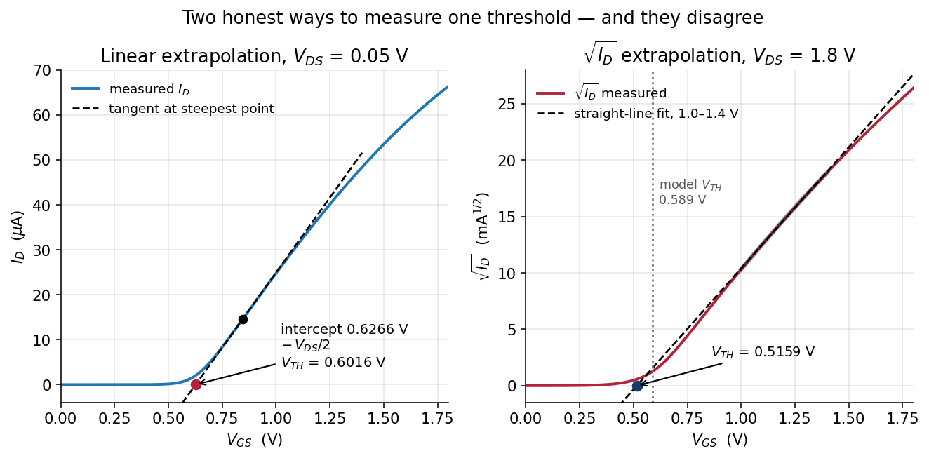
Both panels show a SKY130 nfet_01v8 with W = 5 µm and L = 1 µm, simulated with spice/id_vgs.spice in the Lab 03 package.
Method 1: linear extrapolation at small \(V_{DS}\)
Hold the drain at 0.05 V, which keeps the device firmly in triode where it behaves like a resistor, and sweep the gate. In triode with a small \(V_{DS}\), the current is very nearly a straight line in \(V_{GS}\):
\[I_D \approx \mu_n C_{ox}\frac{W}{L}\left(V_{GS}-V_{TH}-\frac{V_{DS}}{2}\right)V_{DS}\]
Find the steepest point of the measured curve, draw the tangent there, extend it down to \(I_D = 0\), and read off where it crosses. According to the equation, that intercept is \(V_{TH} + V_{DS}/2\), so you subtract half the drain voltage to get \(V_{TH}\). Lab 03’s extraction prints each step of the working:
== V_TH by linear extrapolation   (V_DS = 0.05 V)
   steepest point      V_GS = 0.845 V
   tangent slope       66.716 uA/V
   tangent hits zero   V_GS = 0.6266 V
   minus V_DS/2        V_TH = 0.6016 V
That gives 0.6016 V from four lines of arithmetic on 361 sampled points, without a datasheet.
Method 2: \(\sqrt{I_D}\) extrapolation in saturation
The saturation law says \(I_D \propto (V_{GS}-V_{TH})^2\), so \(\sqrt{I_D}\) should be a straight line whose x-intercept is \(V_{TH}\). Sweep the gate with the drain at 1.8 V, take the square root of the current, fit a line over a sensible window, and extrapolate it to zero:
== V_TH by sqrt(I_D) extrapolation   (V_DS = 1.8 V, fit 1.0-1.4 V)
   sqrt(I_D) slope     21.4889 mA^0.5 / V
                       V_TH = 0.5159 V
This method gives 0.5159 V.
Two methods, 86 mV apart
== your number vs the model's own number   (device A)
   quantity                              yours    ngspice   diff
   V_TH  (linear extrapolation)         0.6016     0.5895   V   +2.07 %
   V_TH  (sqrt extrapolation)           0.5159     0.5895   V  -12.49 %
The ngspice column is @m.xma.msky130_fd_pr__nfet_01v8[vth], the threshold that BSIM itself reports at that operating point, read from spice/op_params.spice. So two reasonable methods and the model, all looking at one device, give three answers spread over 86 mV.
All three are legitimate, because \(V_{TH}\) is defined by its extraction method. The methods disagree because the square law they both rely on isn’t exactly true for this device. Method 1 relies on it only very near threshold, where it is nearly right, and lands within about 2 % of the model. Method 2 relies on it across a whole volt of overdrive, where it is well off, and comes out 12 % low.
Ask how a threshold was extracted. “0.52 V” and “0.60 V” can describe the same transistor, so a datasheet threshold with no method beside it has a tolerance you can’t see.
For the rest of this course we take \(V_{TH} = 0.6016\) V for this device, because that is what the linear extrapolation gives, and every prediction below is checked against it.
The measured knee
Take the five output curves and find where each one stops rising. Lab 03’s src/mosfit.py uses one explicit rule, and says which rule it is: the knee is the first \(V_{DS}\) at which the slope has fallen to 10 % of the slope at the origin. The 10 % is our choice rather than anything physical, and what matters is that the same rule is applied to every curve.
   knee of each curve vs the model's vdsat
     V_GS  V_GS - V_TH  your knee     vdsat
     0.60       -0.002       0.09     0.065
     0.90        0.298       0.29     0.256
     1.20        0.598       0.50     0.442
     1.50        0.898       0.70     0.612
     1.80        1.198       0.89     0.779
Read the second and third columns together, from top to bottom.
At \(V_{GS} = 0.9\) V the textbook boundary predicts a knee at 0.298 V, and the curve knees at 0.29 V, so at low overdrive the simple theory is right to two digits.
At \(V_{GS} = 1.8\) V the boundary predicts 1.198 V, but the curve knees at 0.89 V, which makes the theory 35 % higher than the measured knee. Taken the other way round, with \(V_{ov}\) as the base, the knee is 26 % lower than the theory. The error grows steadily the harder you drive the gate.
Velocity saturation
The square law rests on an assumption that is rarely stated: that the drift velocity of the electrons is proportional to the electric field, without limit, so that doubling the field doubles their speed.
In silicon that holds only up to roughly \(10^4\) V/cm. Above that the carriers stop speeding up, because they scatter off the crystal lattice as fast as the field can accelerate them, and they settle at a saturation velocity of about \(10^7\) cm/s. Once the carriers in the channel are moving as fast as they can, more drain voltage can’t push any more current through. This is velocity saturation.
As a result, the current doesn’t wait for \(V_{DS}\) to reach the overdrive \(V_{ov} = V_{GS} - V_{TH}\) before it stops responding. It stops as soon as the field along the channel is high enough, and for \(L = 1\ \mu\mathrm{m}\) and a volt of overdrive, that happens at a lower drain voltage. The model reports the drain voltage where it actually happens as vdsat, and vdsat is below \(V_{ov}\) at every one of the five bias points above.
There are two consequences you’ll use constantly:
- A short device saturates earlier, because the same overdrive across a shorter channel makes a higher field. At \(V_{GS} = 1.8\) V,
spice/op_params.spicegivesvdsat = 0.912V for L = 2 µm andvdsat = 0.362V for L = 0.15 µm. The minimum-length device pinches off at 40 % of the drain voltage the long one needs. - The square law drifts toward a straight line. When the device is fully velocity-saturated, \(I_D\) becomes proportional to \(V_{ov}\) rather than \(V_{ov}^2\). That is why Method 2 under-read the threshold by 12 %: it fitted a square root to a curve that was drifting toward linear.
When a square-law calculation is tens of percent out on a short modern device, suspect the square law before your arithmetic. Simulate the circuit, and use the hand calculation for direction (“wider means more current”) and the simulator for magnitude.
Channel-length modulation
The right-hand end of the \(V_{GS} = 1.8\) V curve isn’t horizontal. The current rises from 682.502 µA at \(V_{DS} = 1.2\) V to 696.275 µA at 1.8 V, which is 2.0 % more current for 0.6 V more on the drain.
You can see the reason in panel 4 of the channel cross-section. As \(V_{DS}\) grows, the pinch-off point moves further from the drain, so the conducting part of the channel gets slightly shorter, and a shorter channel carries more current. This is channel-length modulation, and it is what the \((1 + \lambda V_{DS})\) factor in your textbook approximates.
The slope of the curve in this region is called the output conductance \(g_{ds}\), and its reciprocal is the output resistance \(r_o\):
| Device | \(g_{ds}\) at \(V_{GS}=V_{DS}=1.8\) V | \(r_o = 1/g_{ds}\) |
|---|---|---|
| W = 5 µm, L = 1 µm | 15.593 µS | 64.13 kΩ |
| W = 1 µm, L = 0.15 µm | 51.415 µS | 19.45 kΩ |
Both rows are from spice/op_params.spice. They mean that a saturated transistor isn’t an ideal current source: it behaves like one with 64 kΩ in parallel, or 19 kΩ if you use the minimum-length device.
That resistance sets how much voltage gain one transistor can give, and it is the first thing Transconductance and output resistance uses.
You’ll reproduce every number on this page in Lab 03, Parts 2 and 3.
Check yourself
- Method 1 subtracts \(V_{DS}/2\) from the tangent’s intercept. Where does that term come from?
- Why does Method 2 give a lower \(V_{TH}\) than Method 1 on this device?
- At \(V_{GS}\) = 1.5 V, how far is the measured knee below \(V_{GS} - V_{TH}\), in percent?
- You shorten a device from L = 1 µm to L = 0.15 µm at the same bias. Does
vdsatgo up or down, and does \(r_o\) go up or down?
Next: Lab 03: MOSFET regions.