Linearity and superposition
Between ECE110 and AD102 you learned methods that solve any circuit you were shown. This page explains why adding a single diode breaks those methods, and what still works once it does.
Superposition, Thévenin equivalents, node-voltage analysis with a matrix and the impedance algebra you do in your head are theorems rather than facts about wires, and every one of them rests on the same hypothesis: every element in this circuit is linear. You have never had to check that hypothesis, because until now it has always been true. When it fails, the theorem doesn’t apply at all, and the answer it gives you is wrong rather than approximately right.
What linear means
An element is linear if the relationship between the voltage across it and the current through it keeps two promises:
- Scaling. If you double the voltage, the current doubles too.
- Additivity. The response to \(v_1 + v_2\) is the response to \(v_1\) plus the response to \(v_2\).
A resistor, including the poly-silicon strips you sized in AD102, keeps both, because \(i = v/R\) and division distributes over addition. Capacitors and inductors keep both too, because differentiation and integration are linear operations. Superposition is just additivity applied to a whole circuit at once.
That gives you a direct test for any component: drive it with A, then with B, then with A+B, and see whether the third answer is the sum of the first two.
The additivity test
Lab 02’s spice/straight_line.spice runs exactly that test. It builds six one-ports, three copies each of a 100 kΩ resistor and a 1 µm² SKY130 diode, and drives the three copies of each part at 0.35 V, at 0.35 V again, and at 0.70 V, which is the sum of the first two. These are its results:
| A (0.35 V) | B (0.35 V) | A + B, predicted | A + B, measured at 0.70 V | |
|---|---|---|---|---|
| 100 kΩ resistor | 3.500000 µA | 3.500000 µA | 7.000000 µA | 7.000000 µA |
| 1 µm² diode | 125.4090 pA | 125.4090 pA | 250.8180 pA | 3.917437 µA |
For the resistor, 3.500000 µA + 3.500000 µA = 7.000000 µA, and the measured answer is 7.000000 µA, to seven digits, which is what you’d expect from a theorem whose hypothesis holds.
For the diode, superposition predicts 250.8180 pA, but the circuit actually delivers 3.917437 µA, which is out by a factor of 15,618.6.
Nothing about the wrong answer looks broken. It’s a clean, plausible-looking number with seven significant figures and no noise on it, and nothing in the output says “superposition does not apply”, so it’s up to you to know when the theorem holds and when it doesn’t.
Check before you reach for a linear tool. Before you write down a Thévenin equivalent, a superposition sum or an impedance divider, ask whether every element in the loop is linear. If the loop has even one diode, one transistor or anything else with a curve in it, the answer is no.
You’ll run this test yourself in Lab 02, Part 2.
The diode on linear axes
Here is the same diode swept from −1 V to +0.9 V and plotted the way you have plotted everything so far, as current against voltage with both axes linear.
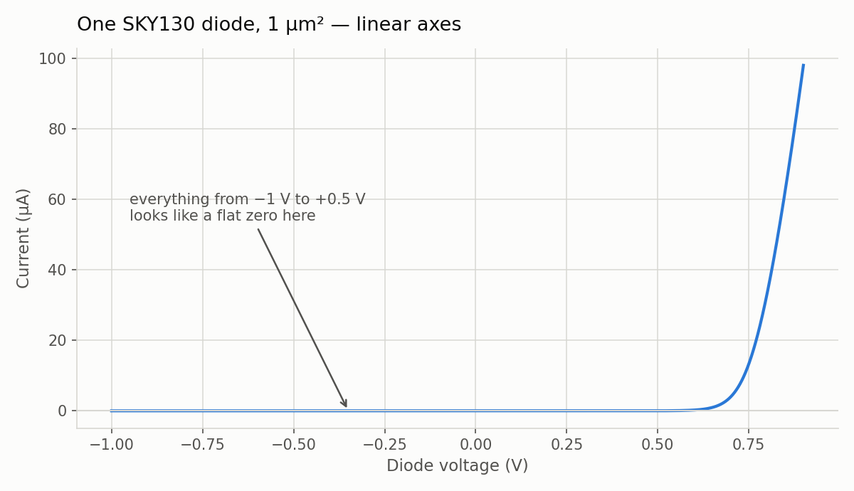
Produced by src/plot_iv.py in the Lab 02 package, from the 1901 rows that spice/diode_iv.spice writes.
On these axes a resistor is a straight line through the origin with slope \(1/R\). The diode is instead a flat stretch followed by a wall. The slope is the conductance, so this component’s resistance is anywhere between “infinite” and “almost zero” depending on where you are on the curve, which means \(R\) is no longer a property of the part.
The current along the flat stretch isn’t zero, though. At −1.000 V the sweep reads −1.003559 pA, and at +0.350 V it reads 125.4090 pA, which is 125 times more current, yet on this plot both are indistinguishable from the axis. Linear axes hide the part of the curve that carries most of the physics, and The diode equation shows it on a better axis.
What still works
Kirchhoff’s laws still hold, because KCL is charge conservation and KVL is energy conservation. Neither law says anything about what the elements are made of, so it makes no difference that one of them is a diode, and you can still write every node equation you know how to write.
| Tool | Still valid with a diode in the loop? |
|---|---|
| KCL, KVL | Yes. They are conservation laws, not linearity results. |
| Ohm’s law on the resistors | Yes. The resistors are still resistors. |
| Superposition | No. It was off by 15,618.6× in the test above. |
| Thévenin / Norton equivalent | No for the part of the circuit containing the diode. It still works for the linear part around the diode, and that turns out to be useful. |
| Series/parallel combination | No for the diode, because it has no \(R\) to combine. |
| Solving the system by algebra | Usually no. You get an equation with \(v\) both inside and outside an exponential, and no rearrangement gets \(v\) on its own. |
The last row is the hard one, and it’s a problem with the equations rather than with diodes. The next page deals with it.
From procedure to search
Until now you have treated circuit analysis as a procedure: identify the topology, apply the right theorem, turn the crank and get a number. For linear circuits that’s the right way to work, and it will serve you for the rest of your career.
With a nonlinear element in the circuit, analysis becomes a search. Instead of asking “what is the answer?”, you ask “which pair of numbers, one voltage and one current, satisfies both the element and the rest of the circuit at the same time?” Instead of a crank to turn, you have a target, and you need a way of closing in on it.
Check yourself
- A circuit contains only resistors, capacitors and inductors. Can you use superposition on it? Why?
- Using the table above, how would you show that a diode fails the scaling promise as well as the additivity one?
- Why can’t you combine a diode in series with a resistor into one equivalent resistance?
Next: The operating point.