Sizing with W and L
When you place a resistor you give it a resistance, and when you place a capacitor you give it a capacitance, but a transistor has no single value like that. Instead you choose two lengths, its width \(W\) and its length \(L\).
Every equation in the last few pages has a factor of \(W/L\) in it, and that is the only factor in them you control. \(\mu_n\), \(C_{ox}\) and \(V_{TH}\) are set by the foundry and come fixed in the model file, and \(V_{GS}\) and \(V_{DS}\) are set by the rest of the circuit. \(W\) and \(L\) are the two numbers you type in, so designing a transistor comes down to choosing them. It’s the lesson AD102 taught you about resistors, that on a chip a value is a geometry, applied to the device that matters most.
Four shapes at one bias
In Lab 03, Part 6, spice/wl_sweep.spice put four differently shaped transistors at the same bias, \(V_{GS} = V_{DS} = 1.8\) V:
| \(W\) | \(L\) | \(W/L\) | why it is there | |
|---|---|---|---|---|
| A | 5 µm | 1 µm | 5 | the reference device from the last few pages |
| B | 10 µm | 1 µm | 10 | twice as wide |
| C | 5 µm | 2 µm | 2.5 | twice as long |
| D | 1 µm | 0.15 µm | 6.67 | minimum length |
If current scaled with \(W/L\), then relative to A, B would carry 2.00× as much current, C would carry 0.50×, and D (whose \(W/L\) is 6.67 against A’s 5) would carry 1.33×, or 928 µA. Here is what the simulation measured:
== W/L is a knob   (V_GS = 1.8 V, V_DS = 1.8 V)
   device              W/L          I_D  I_D/I_D(A)  (W/L)/(W/L)_A
   A  W=5   L=1       5.00   696.275 uA      1.0000         1.0000
   B  W=10  L=1      10.00  1395.320 uA      2.0040         2.0000
   C  W=5   L=2       2.50   380.728 uA      0.5468         0.5000
   D  W=1   L=0.15    6.67   501.046 uA      0.7196         1.3333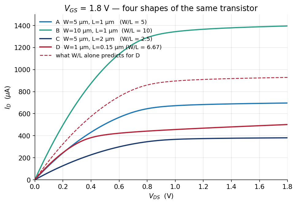
The data are from spice/wl_sweep.spice, plotted by src/plot_curves.py. The dashed line is what \(W/L\) alone predicts for device D, and the solid red curve is what device D actually carries.
The prediction holds for B and misses for C and D, and the two misses have different causes. We’ll take the devices in order of how far off the prediction is, so B comes first.
Device B: width
The prediction for B was 1 392.551 µA and the simulation measured 1 395.320 µA, so the two agree to two parts in a thousand.
That’s because width really is a simple multiplier. Doubling \(W\) is physically the same as putting two of the original transistors side by side and wiring them in parallel, and that is how a wide device is laid out on a real chip anyway, as nf fingers of a narrower device. Nothing about the physics along the channel changes, so the current per micron of width doesn’t change either.
The 0.20 % that’s left over comes from the source and drain diffusion resistance, which doesn’t scale quite in step with \(W\). You’ll meet it properly in AD104, when you draw one of these devices.
So current is proportional to \(W\), and that’s a rule you can trust in hand calculations.
Device C: length
For C the prediction was 348.138 µA and the simulation measured 380.728 µA, so the long device carries 9.4 % more current than \(1/L\) says it should. Two effects add current here.
The threshold. spice/op_params.spice gives C a model vth of 0.5495 V against A’s 0.5895 V (the table under Device D below lists both), so at the same gate voltage C has 40 mV more overdrive. That’s the same trend What moves the threshold measured over nine lengths, seen from the long end. If you put each device’s own threshold into the square law, you get
\[\frac{I_D(\mathrm{C})}{I_D(\mathrm{A})} = \frac{(W/L)_\mathrm{C}\,(1.8-0.5495)^2}{(W/L)_\mathrm{A}\,(1.8-0.5895)^2} = \frac{2.5 \times 1.5638}{5 \times 1.4654} = 0.5336\]
\[696.275\ \mu\mathrm{A} \times 0.5336 = 371.5\ \mu\mathrm{A}\]
which closes about 72 % of the gap between the 348 µA prediction and the measured 381 µA.
The field. As Where saturation starts explained, a longer channel with the same voltage across it has a lower field, so its carriers are further from their speed limit. Expecting the current to halve when you double \(L\) assumes that carrier velocity is proportional to the field without limit, so that half the field gives half the speed. Carriers near their speed limit don’t slow down in proportion when the field drops, so doubling \(L\) costs less than half the current. The measured current is 380.728 / 371.5 = 1.025 times the corrected prediction, and that remaining 2.5 % is this effect.
The model’s own numbers agree. vdsat is 0.912 V for the L = 2 µm device and 0.779 V for L = 1 µm, which means the longer device needs more drain voltage before its carriers stop responding, and that’s another way of saying it was less limited by velocity all along.
The rule you can trust here is that current goes up when you shorten the channel, but by less than \(1/L\) predicts. For quick reasoning, \(1/L\) gets the direction right and overestimates the size of the change.
Device D: minimum length
For D the prediction was 928.367 µA and the simulation measured 501.046 µA, only 54 % of the prediction.
The prediction assumed that \(V_{TH}\) and \(\mu_n\) stay the same when you change the device’s shape, and neither of them does. We can account for the gap in two steps.
Step 1: the threshold moved. spice/op_params.spice gives each device’s threshold at the same bias:
| \(L\) | model vth |
|
|---|---|---|
| A | 1 µm | 0.5895 V |
| C | 2 µm | 0.5495 V |
| D | 0.15 µm | 0.7693 V |
The minimum-length device’s threshold is 180 mV higher than A’s. That is the reverse short-channel effect from What moves the threshold, which showed the same trend over nine lengths at low drain voltage, with the threshold rising at every step to a total of 171 mV. The halo implants that cause it take up a small fraction of a long channel but most of a 0.15 µm one, which is why nfet_01v8 at minimum length is deliberately harder to turn on.
A higher threshold uses up a lot of the overdrive. If you redo the prediction with each device’s own threshold and the square law, you get:
\[\frac{I_D(\mathrm{D})}{I_D(\mathrm{A})} = \frac{(W/L)_\mathrm{D}\,(1.8-0.7693)^2}{(W/L)_\mathrm{A}\,(1.8-0.5895)^2} = \frac{6.667 \times 1.0624}{5 \times 1.4654} = 0.9666\]
\[696.275\ \mu\mathrm{A} \times 0.9666 = 673.06\ \mu\mathrm{A}\]
That brings the prediction down from 928 µA to 673 µA, which is much closer to the measured 501 µA.
Step 2: the carriers hit their speed limit. The measured current is 501.046 / 673.06 = 0.744 of the corrected prediction, and the remaining 26 % is velocity saturation. The model shows it: vdsat for device D is 0.362 V, while its overdrive \(V_{GS} - V_{TH}\) is 1.031 V, so the device stopped responding to drain voltage at barely a third of the overdrive the square law assumed it would use.
So making the transistor 6.7× shorter gives you 0.72× the current instead of 1.33×, because you paid 180 mV of threshold for it and the carriers were already at their speed limit.
This is the most common failure in a first analog design: a hand calculation says the circuit works, a simulation says it doesn’t, and a minimum-length device turns out to be behind the difference. Analog designers usually pick \(L\) two to four times the minimum, and you can now see all three reasons for it: the square law still roughly holds, \(V_{TH}\) is closer to nominal, and \(r_o\) is larger (64.13 kΩ against 19.45 kΩ, or 3.3×, from Where saturation starts). Digital designers use minimum length for the opposite reason, because they want the smallest, fastest switch and they don’t care about \(r_o\).
When a measured current disagrees with \(W/L\) scaling, look at the model’s
vthandvdsatfor that device before you look at your algebra. Two
What geometry costs
You can build \(W/L = 5\) as W = 5 µm, L = 1 µm, or as W = 0.75 µm, L = 0.15 µm. The ratio is the same, so every equation on these pages treats the two identically, but the first one takes up forty-four times the area (5 µm² against 0.1125 µm²).
| Device | \(W \times L\) | area, relative to D |
|---|---|---|
| A | 5 × 1 | 33.3× |
| B | 10 × 1 | 66.7× |
| C | 5 × 2 | 66.7× |
| D | 1 × 0.15 | 1× |
Area costs money. A wafer costs what it costs, and you are billed for the square millimetres you occupy, so every micron of \(W\) you spend buying current is a micron you can’t spend on something else. Area isn’t the only cost, either, because gate capacitance also scales with \(W \times L\). The 30.56 fF from How a MOSFET works is for device A, and every femtofarad of gate has to be charged by whatever drives it, which costs time and energy elsewhere in the circuit.
Designing a transistor means making that trade: more current, with more area and more capacitance, or less of all three. There’s no correct answer to it in general, so it’s a choice you make for each design.
Lab 04 tests the \(W/L\) rule over a much wider range, with seventeen devices, five of which all have \(W/L\) = 5. The second Lab 03 extension (device D at L=0.5) checks whether the two-step arithmetic above still accounts for the whole gap in a longer device.
Check yourself
- Why is doubling \(W\) almost exactly the same as using two devices in parallel?
- Device C is twice as long as A. Why does it carry more than half of A’s current?
- In the two-step calculation for device D, which step closed more of the gap?
- Two designs have \(W/L\) = 5, one at minimum length and one at L = 1 µm. Name one property the long one wins on and one it loses on.
Next: Lab 04: Testing the W/L rule.