Lab 03: MOSFET regions
You’ll sweep a real SKY130 nfet_01v8 and find cutoff, triode, saturation and subthreshold on your own curves. You’ll extract its threshold voltage two ways and see them disagree by 86 mV, measure \(g_m\) as the slope of a curve, and test whether current really scales with \(W/L\). Then you’ll add a sixth gate voltage to the sweep deck yourself.
Package: labs/lab-03-mosfet-regions/
Before you start
Finish Lab 02.
Read How a MOSFET works, The four regions and Where saturation starts.
Open a terminal in the workbench and go to the lab folder:
cd /foss/designs/modules/ad103/labs/lab-03-mosfet-regionsThe
MakefilesetsPDK=sky130Aitself, so no other setup is needed. For the optional XSchem part at the end, load the environment first (. /foss/designs/common/.designinit).
Time: about 2.25 hours, not counting the optional Part 9. make takes about 50 seconds; the other targets take a few seconds each once make has run, or about ten seconds when they run a deck of their own.
The equations from the guide pages, for reference:
\[ I_D^{\text{tri}} = \mu_n C_{ox}\frac{W}{L}\Big[(V_{GS}-V_{TH})V_{DS} - \tfrac{1}{2}V_{DS}^2\Big] \qquad I_D^{\text{sat}} = \tfrac{1}{2}\mu_n C_{ox}\frac{W}{L}(V_{GS}-V_{TH})^2 \]
with the boundary at \(V_{DS} = V_{ov} = V_{GS} - V_{TH}\). The two slopes are
\[ g_m = \frac{\partial I_D}{\partial V_{GS}} \qquad r_o = \left(\frac{\partial I_D}{\partial V_{DS}}\right)^{-1} \]
and below threshold, where the square law doesn’t apply, the subthreshold slope \(S = \partial V_{GS} / \partial (\log_{10} I_D)\), in mV/decade, describes the exponential.
Part 1: Run the sweeps
Does your workbench reproduce the reference sweeps?
Run the four sweeps and the operating-point dump, and check the results:
make== sweeping spice/id_vds.spice wrote results/id_vds.txt == sweeping spice/id_vgs.spice wrote results/id_vgs.txt == sweeping spice/id_vgs_log.spice wrote results/id_vgs_log.txt == sweeping spice/wl_sweep.spice wrote results/wl_sweep.txt == operating point spice/op_params.spice wrote results/op_params.log == checking YOUR NUMBERS ok I_D from id_vds.txt, V_GS=1.8 V 696.2755 uA (reference 696.2750) ok I_D W=5 L=1, V_GS=V_DS=1.8 V 696.2755 uA (reference 696.2750) ok I_D W=10 L=1, same bias 1395.3199 uA (reference 1395.3200) ok I_D W=5 L=2, same bias 380.7284 uA (reference 380.7280) ok I_D W=1 L=0.15, same bias 501.0462 uA (reference 501.0460) ok V_TH by linear extrapolation 0.6016 V (reference 0.6016) ok V_TH by sqrt(I_D) extrapolation 0.5159 V (reference 0.5159) ok g_m at V_GS = 1.8 V 914.6500 uS (reference 914.6500) ok subthreshold slope 85.5629 mV/dec (reference 85.6000) PASS all nine extracted parameters match the reference runIf any line says
XX,check.pytells you which one and lists the four things that most often cause it, most frequent first.Draw the plots into
results/:make figuresIt writes six PNGs plus the channel cross-section figure. Open them as you go through the parts below.
Print every extracted parameter with its working. You’ll read this output block by block in Parts 2 to 6:
make extract
You should see PASS all nine extracted parameters match the reference run, and seven PNG files in results/.
Part 2: Extract the threshold two ways
What is \(V_{TH}\) for this device?
Open
results/ad103-vth-extraction.png: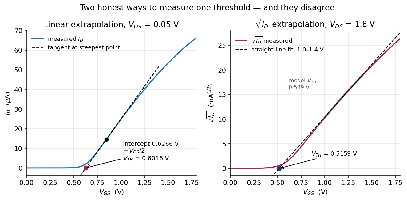
Two threshold extractions side by side Find the two
V_THblocks in themake extractoutput: linear extrapolation at \(V_{DS}\) = 0.05 V, and \(\sqrt{I_D}\) extrapolation at \(V_{DS}\) = 1.8 V.Find the model’s own threshold for the same device in the operating-point log:
grep -i 'xma.*\[vth\]' results/op_params.logxmais device A inspice/op_params.spice, the same W = 5 µm, L = 1 µm transistor. Compare all three with theyour number vs the model's own numberblock near the end of themake extractoutput.
You should see 0.6016 V by linear extrapolation, 0.5159 V by \(\sqrt{I_D}\) extrapolation and 0.5895 V from the model. That’s three different answers for one device, spread over 86 mV. Use 0.6016 V as \(V_{TH}\) for the rest of this lab.
Which of the three is the right threshold, and why do they disagree?
None of them is wrong, because \(V_{TH}\) is defined by the method you use to extract it. The two extraction methods disagree because both rely on the square law, and the square law isn’t exactly true for this device. Linear extrapolation relies on it only very near threshold, so it lands 2.07 % from the model. \(\sqrt{I_D}\) extrapolation relies on it across a whole volt of overdrive, so it ends up 12.49 % out. Where saturation starts goes through this in more detail.
Part 3: The output characteristic
Where does each output curve knee, and does it land at \(V_{GS} - V_{TH}\)?
Open
results/ad103-id-vds-family.png: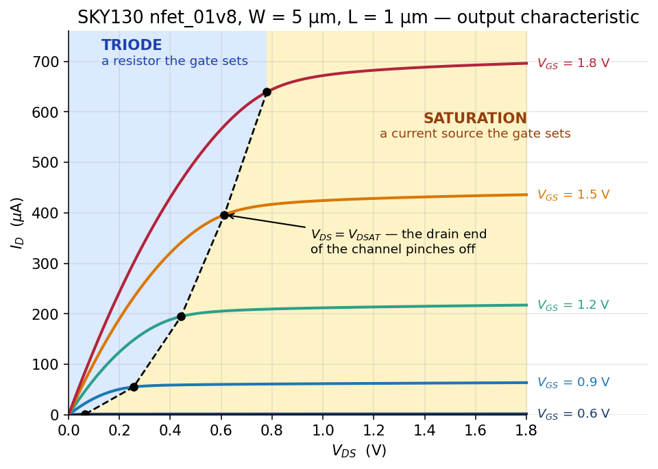
I_D vs V_DS for five gate voltages, with the regions shaded Read the first block of
make extract,I_D vs V_DS. Look first at thechannel R at V_DS=10 mVcolumn, which gives the channel’s resistance at each gate voltage.Work out \(V_{GS} - V_{TH}\) for the 0.9 V to 1.8 V curves, using your \(V_{TH}\) of 0.6016 V, and compare it with the
knee V_DScolumn. Then find theknee of each curve vs the model's vdsattable at the end of the output.Find the lowest current in the
below thresholdblock: \(V_{GS}\) = 0 V, with 1.8 V on the drain.
You should see the channel resistance fall from 26.6 kΩ to 737 Ω as \(V_{GS}\) goes from 0.6 V to 1.8 V. At \(V_{GS}\) = 0.9 V the knee lands at 0.29 V against a predicted 0.298 V, which is close, but at 1.8 V it lands at 0.89 V against a predicted 1.198 V, so there the prediction is 35 % high. The model’s vdsat is below \(V_{GS} - V_{TH}\) at every gate voltage. Even with the gate at 0 V, the device still passes 2.1853 pA.
Why does the 1.8 V curve knee so far below \(V_{GS} - V_{TH}\)?
The cause is velocity saturation. The square law assumes that carrier speed keeps rising with the electric field, but above roughly \(10^4\) V/cm the carriers stop speeding up. Once they’re moving as fast as they can, more drain voltage adds nothing, so the current stops responding before \(V_{DS}\) reaches \(V_{ov}\). The harder you drive the gate, the bigger the error, which is why the 0.9 V curve lands close to its prediction and the 1.8 V curve doesn’t. See Where saturation starts.
Part 4: Subthreshold conduction
Is a transistor below threshold really off?
Write down what you predicted for \(I_D\) at \(V_{GS}\) = 0.30 V when you read The four regions. If you skipped the prediction, make one now.
Read the
below thresholdblock ofmake extract, and openresults/ad103-subthreshold.png: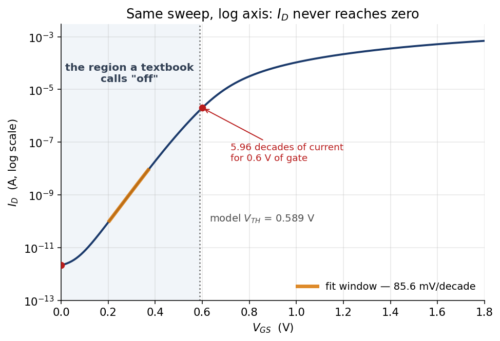
I_D vs V_GS on a log axis Multiply the \(V_{GS}\) = 0 V current by ten million transistors. Then do the same with the \(V_{GS}\) = 0.30 V current, which is what a device with a threshold 0.3 V lower would carry with its gate at ground.
You should see 1.3645 nA at \(V_{GS}\) = 0.30 V, which is small but not zero. On the log plot it sits on a straight line 5.96 decades tall, with a slope of 85.6 mV/decade. Ten million transistors at 2.1853 pA each add up to 21.9 µA of leakage, and the same ten million with a threshold 0.3 V lower draw 13.6 mA.
The two leakage totals are a factor of 624 apart. What does that say about how a process has to treat its threshold voltage?
A threshold 0.3 V lower multiplies the leakage of those ten million transistors by 624, from 21.9 µA to 13.6 mA. Because a shift that small changes a chip’s leakage that much, a process has to hold its threshold voltage tightly, and threshold control is a discipline of its own.
Part 5: Measure \(g_m\) two ways
Does the slope of your sweep agree with the \(g_m\) the model reports?
Open
results/ad103-gm.png: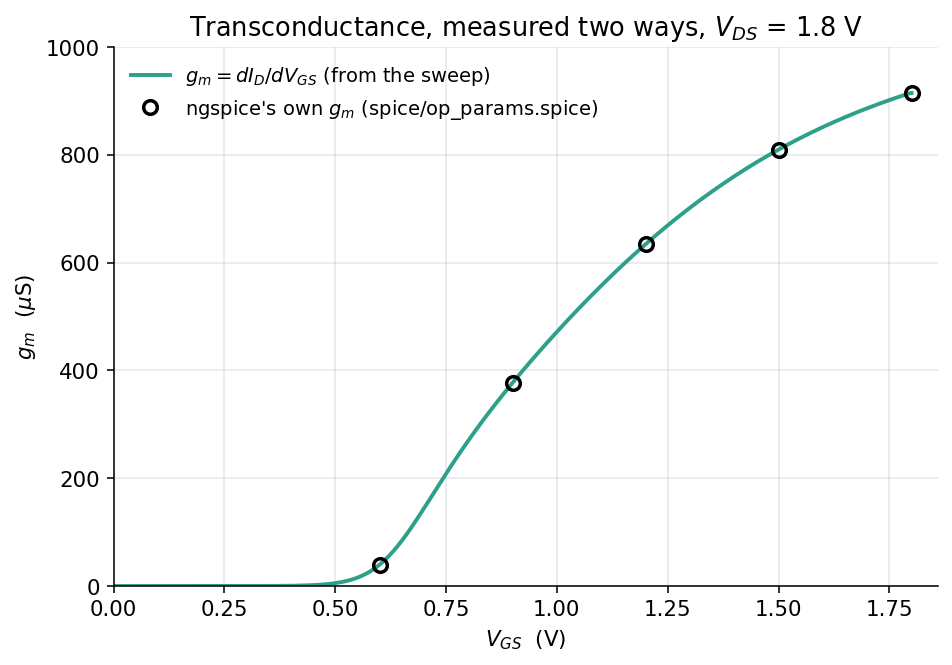
g_m from the sweep, with ngspice’s own g_m overlaid The green curve is
numpy.gradientapplied to your sweep. The circles are the \(g_m\) that ngspice’s model reports at five bias points. The two are computed by completely different means, so each is an independent check on the other.Read the
g_m = dI_D/dV_GSblock ofmake extract, and theg_mline in theyour number vs the model's own numberblock.
You should see 914.650 µS from the slope of your sweep against 915.312 µS from the model at \(V_{GS}\) = 1.8 V, 0.07 % apart. In the g_m/I_D column, the value falls from 5.90 /V at \(V_{GS}\) = 0.9 V to 1.31 /V at 1.8 V.
What does \(g_m/I_D\) measure, and what does its trend say about where to bias an amplifier?
\(g_m/I_D\) is the transconductance you get for each unit of current you burn, so it measures how efficiently the device uses its bias current. It’s highest near threshold and lowest with the gate wide open, which is the opposite of where a beginner tends to bias an amplifier. Transconductance and output resistance, which you’ll read before Lab 04, picks this up.
Part 6: Four device geometries at one bias
Does current scale with \(W/L\)?
The W/L is a knob block puts four devices at \(V_{GS} = V_{DS}\) = 1.8 V:
| \(W\) | \(L\) | \(W/L\) | |
|---|---|---|---|
| A | 5 µm | 1 µm | 5 |
| B | 10 µm | 1 µm | 10 |
| C | 5 µm | 2 µm | 2.5 |
| D | 1 µm | 0.15 µm | 6.67 |
Before you look, use \(W/L\) alone to predict the currents of B, C and D relative to A, which carries 696.275 µA. Write the three numbers down.
Read the
W/L is a knobblock ofmake extract, and openresults/ad103-wl-sweep.png: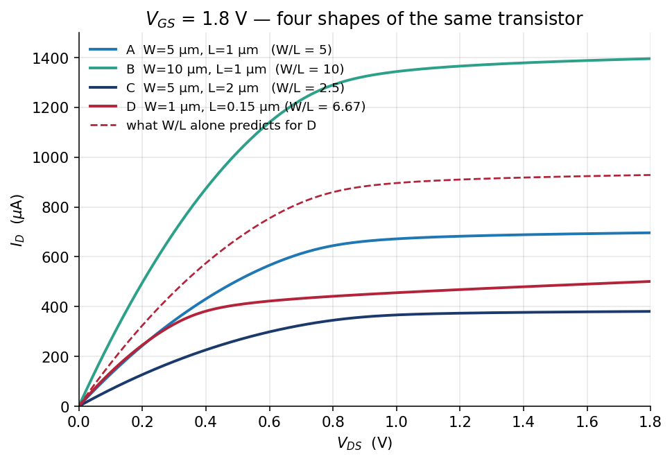
Four device geometries at the same bias For each device, work out how far the measurement is from your prediction, in percent.
You should see B within 0.20 % of twice A’s current, so width scales the way \(W/L\) says it should. Doubling \(L\) gives 9.4 % more current than \(1/L\) predicts, and the minimum-length device D delivers 501.046 µA against a predicted 928.367 µA, only 54 % of the prediction. Sizing with W and L, which you’ll read before Lab 04, closes that gap in two steps.
Part 7: Units on W and L
What does a unit suffix on W do to this deck?
Predict what ngspice will print. You made the same mistake on purpose in Lab 01, Part 6.
Run the deck with units on
WandL:make wrong-unitsError on line 56 or its substitute: m.xm1.msky130_fd_pr__nfet_01v8 d g 0 0 xm1:sky130_fd_pr__nfet_01v8__model l= 1.000000000000000e-06 w= 5.000000000000000e-06 ... could not find a valid modelname Simulation interrupted due to error! Error: incomplete or empty netlist or no ".plot", ".print", or ".fourier" lines in batch mode; no simulations run!Find what changed:
diff spice/id_vds.spice spice/id_vds_wrong_units.spice
You should see that the two decks differ by two characters, the two us in L=1u W=5u where the working deck has L=1 W=5, and that the error message names neither W nor units.
Why does a u make ngspice stop here, when the same u on a diode in Lab 02 ran silently?
SKY130’s MOSFET models are binned in microns: each model covers a range of widths and lengths, so a width with a u on it matches no bin, and ngspice stops. The diode models aren’t binned, so there’s no range for a wrong size to fall outside, and the diode deck runs without complaint.
Part 8: Add a sixth gate voltage
Can you add a curve to spice/id_vds.spice so that the analysis picks it up?
The deck sweeps \(V_{DS}\) once for each gate voltage in its foreach list. You’ll add a curve at \(V_{GS}\) = 1.05 V, which sits between the 0.9 V and 1.2 V curves. It takes four edits.
Predict \(I_D\) at \(V_{GS}\) = 1.05 V and \(V_{DS}\) = 1.8 V from the 0.9 V and 1.2 V rows of the first
make extracttable. Write it down.Open
spice/id_vds.spicein a text editor and add1.05to theforeachline as the second entry, right after0.6. We have you put it there rather than at the end on purpose: at the end, the existingletlines would keep their numbers, and renumbering them in step 3 is the part worth practising.Each
dccommand makes its own plot, nameddc1,dc2, … in the order the sweeps ran. Add aletline for the new curve (call itid_vgs105), and fix thedcNnumbers on the otherletlines to match the new order.TipAnswerThe 1.05 V sweep now runs second, so it is
dc2, and every curve after it moves down by one:let id_vgs06 = -dc1.i(vds) let id_vgs105 = -dc2.i(vds) let id_vgs09 = -dc3.i(vds) let id_vgs12 = -dc4.i(vds) let id_vgs15 = -dc5.i(vds) let id_vgs18 = -dc6.i(vds)The
NindcNcounts sweeps in the order they ran, and has nothing to do with the gate voltage.Add
id_vgs105to thewrdataline, and save the file. Its position in that list doesn’t matter, becauseextract.pymatches each column to its gate voltage through the vector’s name.Run the lab and print the extraction again:
make
make extract
The first table of
make extractnow has six rows. Thegate voltages readline lists the gates in the order of yourwrdataline, so yours may differ from the one below, which hadid_vgs105second. The table under it is sorted by gate voltage either way:== I_D vs V_DS (W=5, L=1) gate voltages read from spice/id_vds.spice: 0.6 1.05 0.9 1.2 1.5 1.8 V_GS I_D at V_DS=1.8 knee V_DS channel R at V_DS=10 mV 0.60 2.005 uA 0.09 V 26648.3 ohm 0.90 63.876 uA 0.29 V 2529.2 ohm 1.05 131.053 uA 0.39 V 1690.0 ohm 1.20 217.505 uA 0.50 V 1288.0 ohm 1.50 436.080 uA 0.70 V 907.7 ohm 1.80 696.275 uA 0.89 V 736.9 ohm
You should see a sixth row, 131.053 µA at \(V_{GS}\) = 1.05 V, sorted into gate-voltage order, and make still printing PASS. That works because nothing in src/ assumes five curves; extract.py reads the gate list back out of the deck. The reference deck is solutions/id_vds_six.spice, and solutions/README.md discusses it.
Part 9 (optional): Draw it in XSchem
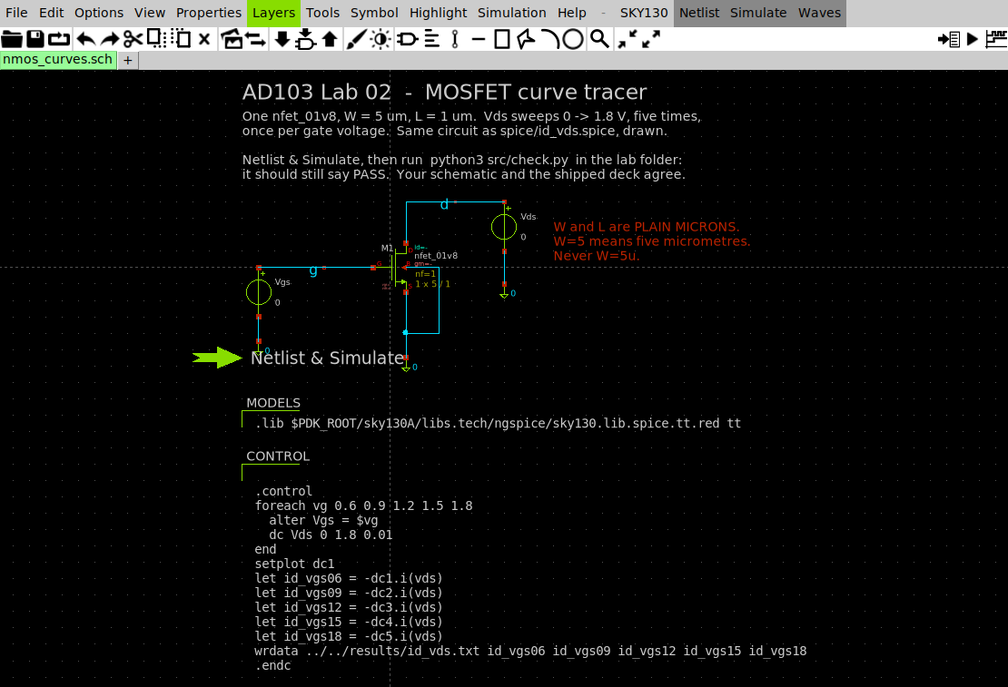
xschem/nmos_curves.sch: the same circuit as the shipped spice/id_vds.spice, drawn. The .lib line and the .control block are carried in two code_shown symbols, which is how a testbench keeps its simulation commands next to its circuit.
Do this part after you’ve finished Part 8 and checked its line in Finishing, because this step throws your Part 8 edit away. The schematic writes five columns, and
check.pyreads the gate list from the deck, so with your six-curve deck in place it reportsthe results file is stale. Putspice/id_vds.spiceback to five curves (your course folder is the git clone from Lab 01’smod add):git checkout -- spice/id_vds.spice makeOpen the schematic:
cd xschem
PDK=sky130A xschem nmos_curves.sch &
Find the green Netlist & Simulate launcher arrow on the canvas. It isn’t a toolbar button, and a plain left-click on it only selects it, without netlisting, simulating or printing any message. Click the arrow once to select it, then press
Ctrl-Hto fire it. (Ctrl-click on the arrow also works, but it misses if your hand drifts between press and release. The XSchem cheat sheet has the same note.)Back in the lab folder, rerun the checker on the data the schematic wrote:
cd ..
python3 src/check.py
You should see PASS again, because the schematic writes the same results/id_vds.txt. The drawn device carries 696.226 µA rather than 696.275 µA, because the XSchem symbol adds the diffusion resistances nrd and nrs that the hand-written deck leaves out. Those resistances come from how the device is laid out, so the 50 nA difference is layout showing up in an electrical answer.
Finishing
You’re done when make extract shows your sixth row, 131.053 µA at \(V_{GS}\) = 1.05 V, and make still prints PASS with your edited deck (Part 8).
Questions
What are the three threshold values for this device, and why do they differ? (Part 2.)
At \(V_{GS}\) = 1.8 V, where does the curve knee, and why is it below \(V_{GS} - V_{TH}\)? (Part 3.)
Which of B, C and D in Part 6 matched your \(W/L\) prediction, and which missed?
TipAnswerB, the wider device, matched to within 0.20 %. C, the longer one, carried 9.4 % more than \(1/L\) predicts, and D, the minimum-length device, carried only 54 % of its prediction.
Submit
Nothing to submit.
Going further
Two more changes to the decks, with reference answers in labs/lab-03-mosfet-regions/solutions/. Try them before you open that folder.
- Repeat it for a PMOS. Do the same measurements for
pfet_01v8and find out how much of this lab is about n-channel devices specifically. - Lengthen the short device. Set device D in
spice/wl_sweep.spicetoL=0.5, rerunmake extract, and watchvth,vdsatand \(I_D\) move together. Check whether the two-step arithmetic in Sizing with W and L still closes.
Next on the Course path: read What moves the threshold.